Bracketed minimization

Like in root finding, you will often have some idea of where the optimum is. In similar fashion, we can iteratively improve our brackets until they are close enough.

Golden section search¶

In the bisection root finding algorithm, two points were sufficient since they identify a sign change. For minimization, we need to determine a minimum, so we need 3 points.

Given 3 points $(x_1, x_2, x_3)$

Choose a point $x_4$

Evaluate the function at $x_4$

If $f(x_4) < f(x_2)$, select $\langle x_2, x_4, x_3 \rangle$.

If $f(x_4) > f(x_2)$, select $\langle x_1, x_2, x_4 \rangle$.

Repeat until a tolerance is met

How do we choose $x_4$?

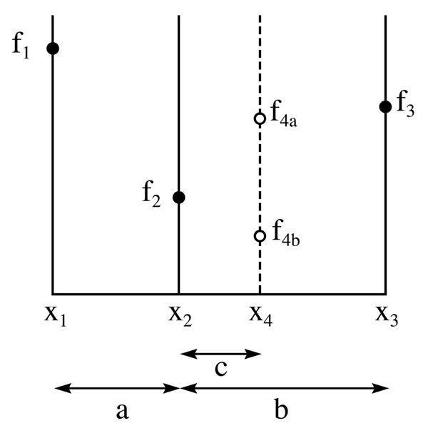
The Golden ratio¶

To make a robust method, we want both of these paths to result in the same reduction of the search interval, and ideally reuse the function evaluations. This self-similarity implies we want to maintain the ratio of subdivision:

In the triplet $\langle x_1, x_2, x_4 \rangle$ with $f_{4a}$, we want $\frac{c}{a}=\frac{a}{b}$.

In the triplet $\langle x_2, x_4, x_3 \rangle$ with $f_{4b}$, we want $\frac{c}{b-c}=\frac{a}{b}$.

Using these two equations, we can eliminate $c$ and find,

and ignoring the negative root,

the Golden ratio!

Convergence rate¶

Each iteration of the Golden section method reduces the bracketed interval by a constant factor of $\varphi^{-1} \approx 0.618$.

The Golden section method is guaranteed to converge, doing so reliably at a linear rate ($k=1$ with rate constant $\varphi^{-1} \approx 0.618$).

Let’s see this on the unimodal function $f(x) = x^4 + 10x$ (where the true minimum is at $x^* = -(10/4)^{1/3} \approx -1.3572$):

Brent’s method¶

We’ve seen this concept before in root finding with bisection. Later we saw the value of using the function values to approximate the derivative and guess at the root. Since we had two points, we fit a line (which approximated the derivative) which is the Secant method.

Now we have 3 points so we can fit a parabola and find $f_{\min} = f(x_{\min})$!

Parabolic interpolation¶

Fitting a parabola through the three points $(x_1, f_1)$, $(x_2, f_2)$, and $(x_3, f_3)$ allows us to jump directly to the vertex of that parabola as our next estimate $x_4$:

(Note: For root finding, where we want $x$ where $f(x)=0$, Brent’s root-finding algorithm uses inverse quadratic interpolation to fit $x(f)$. For minimization, where we want $f'(x)=0$, Brent’s minimization method uses successive parabolic interpolation as written above!)

The convergence order of parabolic interpolation on smooth functions is superlinear ($k \approx 1.325$).

Combination with Golden section¶

Brent’s method combines the robustness of the Golden Section method with the acceleration of parabolic approximation (still without any derivative information!).

Candidate steps from parabolic interpolation and Golden section are generated and compared against various criteria for robustness and progression.

This decision tree makes the exact convergence behavior adaptive, achieving superlinear convergence ($k \approx 1.325$) for well-behaved functions while guaranteeing at least the linear convergence rate of Golden section search.

Example: Unimodal minimization¶

Minimize $f(x) = x^4 + 10x$ using Brent’s method and compare the evaluation count and convergence curve against Golden section search:

Example: Non-differentiable function¶

Let’s try a non-differentiable function: $f(x) = |x|$:

Example: A more treacherous function¶

Minimize $f(x) = |\sin(x)| + |\cos(x)| + 0.1 x^2$