Yet another method involves invoking our interpolator methods to model the solution directly. The process is:
Determine a set of (possibly unevenly spaced) points, .
Define an interpolator function with unknown parameters .
Apply the ODE at each point and find a residual,
Solve (root find or in least squares) for the interpolator parameters.
We can apply a number of interpolators to this scheme, but some common ones include:
Splines (1D / 2D)
Radial Basis Functions (ND)
Neural Networks
Spectral methods
Spectral methods in this context refers to the use of special basis functions (Sin / cos, Chebychev, Legenre polynomials, etc) with associated optimal collocation points.
Pros / Cons
Benefits:
Flexibility: Can handle complex geometries and irregular domains.
High Accuracy: Often provides high accuracy with fewer collocation points, especially with higher-order polynomials.
Versatility: Suitable for a wide range of problems, including ODEs and PDEs.
Spectral Methods: Achieve exponential convergence for smooth problems when using spectral collocation (e.g., Chebyshev or Legendre polynomials).
Drawbacks:
Complexity: More complex to implement compared to FDM, especially for higher-order methods.
Computational Cost: Can be computationally expensive due to the need to solve large systems of equations.
Stability: Requires careful selection of collocation points to ensure stability and convergence.
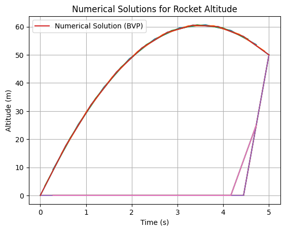
Example: Splines
def fun(x, y):
  plt.plot(x,y[0])
  return np.vstack((y[1], -9.8*np.ones_like(y[1])))

def bc(ya, yb):
  return np.array([ya[0], yb[0] - 50])

x = np.linspace(0, 5, 10)
y = np.zeros((2, x.size))
y[0, 0] = 0
y[0, -1] = 50
sol = solve_bvp(fun, bc, x, y)

# Plot the solution from solve_bvp
plt.plot(sol.x, sol.y[0], label='Numerical Solution (BVP)')
plt.xlabel('Time (s)')
plt.ylabel('Altitude (m)')
plt.title('Numerical Solutions for Rocket Altitude')
plt.legend()
plt.grid(True)
plt.show()
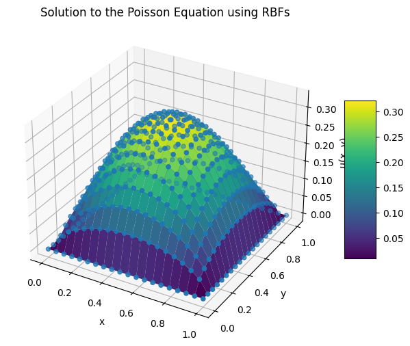
import numpy as np
from scipy.spatial.distance import cdist
import matplotlib.pyplot as plt
from matplotlib import cm

# Parameters
N = 20  # Number of nodes in each direction (NxN grid)
epsilon = N/np.sqrt(2)  # Shape parameter for RBFs

# Define the RBF (we use a Gaussian RBF in this example)
def rbf(r, epsilon):
    return np.exp(-(epsilon * r) ** 2)

# Define the Laplacian of the RBF (for the Poisson equation)
def laplacian_rbf(r, epsilon):
    return (4 * epsilon**2 - 4 * epsilon**4 * r**2) * np.exp(-(epsilon * r) ** 2)

# Generate nodes in a square domain [0,1]x[0,1]
x = np.linspace(0, 1, N)
y = np.linspace(0, 1, N)
X, Y = np.meshgrid(x, y)
points = np.vstack([X.ravel(), Y.ravel()]).T

#points = np.random.uniform(0, 1, (N**2, 2))

# Compute pairwise distance matrix
r = cdist(points, points)

# Build the RBF matrix and Laplacian matrix
A = rbf(r, epsilon)
L = laplacian_rbf(r, epsilon)

# Define right-hand side (RHS) for Poisson equation
rhs = np.full(points.shape[0], 4.0)

# Apply boundary conditions (u=0 on the boundary)
boundary_indices = np.where((points[:, 0] == 0) | (points[:, 0] == 1) |
                            (points[:, 1] == 0) | (points[:, 1] == 1))[0]
interior_indices = np.setdiff1d(np.arange(points.shape[0]), boundary_indices)

# Modify RHS and matrices to incorporate Dirichlet BCs
rhs[boundary_indices] = 0
A[boundary_indices, :] = 0
A[boundary_indices, boundary_indices] = 1
L[boundary_indices, :] = 0
L[boundary_indices, boundary_indices] = 1

# Solve for the weights
weights = np.linalg.solve(L, rhs)

# Calculate solution u as a weighted sum of RBFs
u = A @ weights

# Reshape solution to 2D grid
U = u.reshape(N, N)

fig = plt.figure(figsize=(8, 6))
ax = fig.add_subplot(111, projection='3d')
surf = ax.plot_surface(X, Y, U, cmap=cm.viridis)
ax.scatter(points[:,0], points[:,1], u)
fig.colorbar(surf, shrink=0.5, aspect=5)
ax.set_xlabel("x")
ax.set_ylabel("y")
ax.set_zlabel("u(x, y)")
ax.set_title("Solution to the Poisson Equation using RBFs")
plt.show()