General Runge-Kutta methods - Executable Engineering: Interactive Numerical Methods in Python

We are now in a position to generalize the Runge-Kutta (RK) methods. Our goal is to use intermediate evaluations of the slope function $f$ called stages $k_n$ to better approximate the true integral (via cancelation of higher order corrections in the Taylor series):

y_{i+1} \approx y_i + h \sum_{n=1}^s a_n k_n

(1)

For the explicit family of RK methods, each stage $k_n$ depends only on previously computed stages:

\begin{aligned} k_1 &= f(t_i, y_i) \\ k_2 &= f(t_i + p_2 h, y_i + [q_{21}k_1] h) \\ k_3 &= f(t_i + p_3 h, y_i + [q_{31}k_1 + q_{32}k_2] h) \\ &\;\;\vdots \\ k_s &= f(t_i + p_s h, y_i + [q_{s1}k_1 + q_{s2}k_2 + \cdots + q_{s,s-1} k_{s-1}] h) \end{aligned}

(2)

RK methods are parameterized by:

nodes $p_n$ - the fraction of the current timestep
coupling coefficients $q_{nm}$ that construct new stages
weights $a_n$ - the final combination for the full time step

These constant parameters are characteristic of the specific RK scheme. Note that RK1 is simply the Forward Euler method.

import numpy as np
import plotly.graph_objects as go

try:
    import executable_engineering as exe
except ImportError:
    %pip install -q executable_engineering
    import executable_engineering as exe

Butcher Tableaux¶

Noting that $a_n$ , $p_n$ , and $q_{nm}$ form two vectors of dimension $s$ and an $s \times s$ matrix, RK schemes can be written compactly in a Butcher Tableau. For explicit methods, this takes the form:

\begin{array}{c|ccccc} p_1 & & & & & \\ p_2 & q_{21} & & & & \\ p_3 & q_{31} & q_{32} & & & \\ \vdots & \vdots & & \ddots & & \\ p_s & q_{s1} & q_{s2} & \cdots & q_{s,s-1} & \\ \hline & a_1 & a_2 & \cdots & a_{s-1} & a_s \end{array}

(3)

Notice that the $q_{nm}$ matrix is strictly lower triangular, allowing each stage to be evaluated sequentially. We will later introduce the implicit family of RK methods, where entries appear on and above the diagonal!

For a given order, the values of $a_n$ , $p_n$ , and $q_{nm}$ are derived to match the Taylor series expansion.

Second-Order Runge-Kutta (RK2) Derivation¶

For RK2 methods:

\begin{align} y_{i+1} &= y_i + [a_1 k_1 + a_2 k_2] h \\ &with \\ k_1 &= f(t_i, y_i) \\ k_2 &= f(t_i + p_2 h, y_i + q_{21} k_1 h) \\ \end{align}

(4)

Performing a bivariate Taylor expansion of $k_2$ around $(t_i, y_i)$ :

k_2 = f(t_i, y_i) + p_2 h \frac{\partial f}{\partial t} + q_{21} k_1 h \frac{\partial f}{\partial y} + O(h^2)

(5)

Substituting $k_1$ and $k_2$ into the update for $y_{i+1}$ :

y_{i+1} = y_i + [a_1 + a_2] f(t_i, y_i) h + \left[a_2 p_2 \frac{\partial f}{\partial t} + a_2 q_{21} f(t_i, y_i) \frac{\partial f}{\partial y}\right] h^2 + O(h^3)

(6)

Comparing this against the exact second-order Taylor expansion using the chain rule $f'(t_i, y_i) = \frac{\partial f}{\partial t} + \frac{\partial f}{\partial y} f(t_i, y_i)$ :

y_{i+1} = y_i + f(t_i, y_i) h + \left[\frac{\partial f}{\partial t} + \frac{\partial f}{\partial y} f(t_i, y_i)\right] \frac{h^2}{2} + O(h^3)

(7)

Matching terms yields three equations for four unknowns (1 degree of freedom):

\begin{aligned} a_1 + a_2 &= 1 \\ a_2 p_2 &= \frac{1}{2} \\ a_2 q_{21} &= \frac{1}{2} \end{aligned}

(8)

RK2 Variants: Heun’s, Midpoint, and Ralston’s Methods¶

Any choice of $a_2$ satisfies the second-order conditions and integrates constant, linear, and quadratic trajectories exactly:

Heun’s Method ( $a_2 = \frac{1}{2}$ ): Averages endpoint slopes $k_1 = f(t_i, y_i)$ and $k_2 = f(t_i + h, y_i + k_1 h)$ .
Midpoint Method ( $a_2 = 1$ ): Uses the midpoint slope $k_2 = f\left(t_i + \frac{1}{2}h, y_i + \frac{1}{2} k_1 h\right)$ .
Ralston’s Method ( $a_2 = \frac{2}{3}$ ): Provides a minimum bound on the leading local truncation error:

y_{i+1} = y_i + \frac{h}{3}[k_1 + 2 k_2], \quad k_1 = f(t_i, y_i), \quad k_2 = f\left(t_i + \frac{3}{4}h, y_i + \frac{3}{4} k_1 h\right)

(9)

\text{Heun:} \quad \begin{array}{c|cc} 0 & & \\ 1 & 1 & \\ \hline & \frac{1}{2} & \frac{1}{2} \end{array} \qquad \text{Midpoint:} \quad \begin{array}{c|cc} 0 & & \\ \frac{1}{2} & \frac{1}{2} & \\ \hline & 0 & 1 \end{array} \qquad \text{Ralston:} \quad \begin{array}{c|cc} 0 & & \\ \frac{3}{4} & \frac{3}{4} & \\ \hline & \frac{1}{3} & \frac{2}{3} \end{array}

(10)

differential_equations_module.py

1
2
3
4
5
6
7
8
9
10
11
12
13
14
15
16
17
18
def ralston_method(f, t0, y0, t_end, h):
    t_points = np.arange(t0, t_end + h / 2, h)
    y_points = np.zeros_like(t_points, dtype=float)
    y_points[0] = y0

    for i in range(len(t_points) - 1):
        t_i, y_i = t_points[i], y_points[i]
        k1 = f(t_i, y_i)
        k2 = f(t_i + 0.75 * h, y_i + 0.75 * h * k1)
        y_points[i + 1] = y_points[i] + h * (k1 + 2.0 * k2) / 3.0

    return {
        "t_points": t_points,
        "y_points": y_points,
        "h": h,
        "method": "Ralston's Method (RK2)",
    }

exe.display_source(exe.ralston_method)

def f(t, y):
    return 4.0 * np.exp(0.8 * t) - 0.5 * y

def y_true(t):
    return (4.0 / 1.3) * (np.exp(0.8 * t) - np.exp(-0.5 * t)) + 2.0 * np.exp(-0.5 * t)

fig = exe.plot_ode_comparison(
    (0, 4),
    y_true,
    {
        "Heun's Method (a2 = 1/2)": exe.heun_method(f, 0.0, 2.0, 4.0, 1.0),
        "Midpoint Method (a2 = 1)": exe.midpoint_ode(f, 0.0, 2.0, 4.0, 1.0),
        "Ralston's Method (a2 = 2/3)": exe.ralston_method(f, 0.0, 2.0, 4.0, 1.0),
    },
    title="Comparison of RK2 Variants: Heun's, Midpoint, and Ralston's Methods",
)
fig.show()

Third-Order Runge-Kutta (RK3) Methods¶

A similar derivation follows for RK3 with additional degrees of freedom. Kutta’s classical third-order choice is:

y_{i+1} = y_i + \frac{h}{6}[k_1 + 4 k_2 + k_3]

(11)

with

\begin{aligned} k_1 &= f(t_i, y_i) \\ k_2 &= f\left(t_i + \frac{1}{2}h, y_i + \frac{1}{2} k_1 h\right) \\ k_3 &= f(t_i + h, y_i - k_1 h + 2 k_2 h) \end{aligned}

(12)

which reduces to Simpson’s $1/3$ Rule when $f$ is solely a function of $t$ , achieving $O(h^4)$ local and $O(h^3)$ global accuracy:

\begin{array}{c|ccc} 0 & & & \\ \frac{1}{2} & \frac{1}{2} & & \\ 1 & -1 & 2 & \\ \hline & \frac{1}{6} & \frac{2}{3} & \frac{1}{6} \end{array}

(13)

differential_equations_module.py

1
2
3
4
5
6
7
8
9
10
11
12
13
14
15
16
17
18
19
def rk3_method(f, t0, y0, t_end, h):
    t_points = np.arange(t0, t_end + h / 2, h)
    y_points = np.zeros_like(t_points, dtype=float)
    y_points[0] = y0

    for i in range(len(t_points) - 1):
        t_i, y_i = t_points[i], y_points[i]
        k1 = f(t_i, y_i)
        k2 = f(t_i + 0.5 * h, y_i + 0.5 * h * k1)
        k3 = f(t_i + h, y_i - h * k1 + 2.0 * h * k2)
        y_points[i + 1] = y_points[i] + h * (k1 + 4.0 * k2 + k3) / 6.0

    return {
        "t_points": t_points,
        "y_points": y_points,
        "h": h,
        "method": "Classical RK3",
    }

exe.display_source(exe.rk3_method)

Fourth-Order Runge-Kutta (Classical RK4)¶

Classical RK4 is the workhorse of fixed-step explicit integration:

y_{i+1} = y_i + \frac{h}{6}[k_1 + 2 k_2 + 2 k_3 + k_4]

(14)

with

\begin{aligned} k_1 &= f(t_i, y_i) \\ k_2 &= f\left(t_i + \frac{1}{2}h, y_i + \frac{1}{2} k_1 h\right) \\ k_3 &= f\left(t_i + \frac{1}{2}h, y_i + \frac{1}{2} k_2 h\right) \\ k_4 &= f(t_i + h, y_i + k_3 h) \end{aligned}

(15)

achieving $O(h^5)$ local and $O(h^4)$ global truncation error:

\begin{array}{c|cccc} 0 & & & & \\ \frac{1}{2} & \frac{1}{2} & & & \\ \frac{1}{2} & 0 & \frac{1}{2} & & \\ 1 & 0 & 0 & 1 & \\ \hline & \frac{1}{6} & \frac{1}{3} & \frac{1}{3} & \frac{1}{6} \end{array}

(16)

differential_equations_module.py

1
2
3
4
5
6
7
8
9
10
11
12
13
14
15
16
17
18
19
20
def rk4_method(f, t0, y0, t_end, h):
    t_points = np.arange(t0, t_end + h / 2, h)
    y_points = np.zeros_like(t_points, dtype=float)
    y_points[0] = y0

    for i in range(len(t_points) - 1):
        t_i, y_i = t_points[i], y_points[i]
        k1 = f(t_i, y_i)
        k2 = f(t_i + 0.5 * h, y_i + 0.5 * h * k1)
        k3 = f(t_i + 0.5 * h, y_i + 0.5 * h * k2)
        k4 = f(t_i + h, y_i + h * k3)
        y_points[i + 1] = y_points[i] + h * (k1 + 2.0 * k2 + 2.0 * k3 + k4) / 6.0

    return {
        "t_points": t_points,
        "y_points": y_points,
        "h": h,
        "method": "Classical RK4",
    }

exe.display_source(exe.rk4_method)

def f(t, y):
    return 4.0 * np.exp(0.8 * t) - 0.5 * y

def y_true(t):
    return (4.0 / 1.3) * (np.exp(0.8 * t) - np.exp(-0.5 * t)) + 2.0 * np.exp(-0.5 * t)

fig = exe.plot_ode_comparison(
    (0, 4),
    y_true,
    {
        "Forward Euler (RK1)": exe.forward_euler(f, 0.0, 2.0, 4.0, 1.0),
        "Ralston's (RK2)": exe.ralston_method(f, 0.0, 2.0, 4.0, 1.0),
        "Classical RK3": exe.rk3_method(f, 0.0, 2.0, 4.0, 1.0),
        "Classical RK4": exe.rk4_method(f, 0.0, 2.0, 4.0, 1.0),
    },
)
fig.show()

Example: Geometric Anatomy of RK4 Stages¶

Notice how the RK4 algorithm walks its way forward across the interval: partial trial steps $k_1, k_2, k_3, k_4$ inform subsequent slope evaluations, culminating in a highly accurate weighted step.

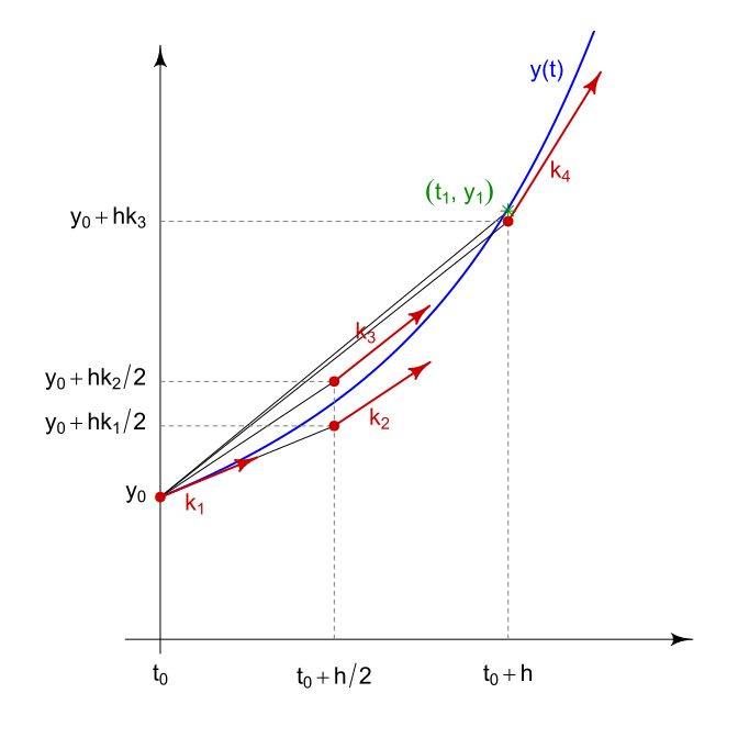
Because internal stages systematically cancel higher-order Taylor derivatives, a single RK4 step achieves far better accuracy than two RK2 half-steps using the same number of function evaluations. However, this assumes the solution is smooth over the step $h$ —when rapid transients occur, we need adaptive time stepping.

fig = exe.plot_rk4_stages(f, y_true, t0=0.0, y0=2.0, h=1.0)
fig.show()