Matrix Types and Sparsity - Executable Engineering: Interactive Numerical Methods in Python

import numpy as np
import matplotlib.pyplot as plt

try:
    import executable_engineering as exe
except ImportError:
    %pip install -q executable_engineering
    import executable_engineering as exe

Common Matrix Types¶

Before discussing advanced structural properties, here is a formal classification of fundamental matrix types encountered in numerical methods:

Matrix Type	Property	Example $2 \times 2$
Zero Matrix	$a_{ij} = 0$ for all $i,j$	$\begin{bmatrix} 0 & 0 \\ 0 & 0 \end{bmatrix}$
Identity Matrix	$\mathbf{A}\mathbf{x} = \mathbf{x}$ , ( $a_{ii}=1, a_{ij}=0$ )	$\begin{bmatrix} 1 & 0 \\ 0 & 1 \end{bmatrix}$
Diagonal	$a_{ij} = 0$ for $i \neq j$	$\begin{bmatrix} 2 & 0 \\ 0 & 3 \end{bmatrix}$
Upper Triangular	$a_{ij} = 0$ for $i > j$	$\begin{bmatrix} 2 & -1 \\ 0 & 3 \end{bmatrix}$
Lower Triangular	$a_{ij} = 0$ for $i < j$	$\begin{bmatrix} 2 & 0 \\ -1 & 3 \end{bmatrix}$
Symmetric	$\mathbf{A} = \mathbf{A}^T$	$\begin{bmatrix} 2 & -1 \\ -1 & 3 \end{bmatrix}$
Positive Definite	$\mathbf{x}^T \mathbf{A} \mathbf{x} > 0$ for all $\mathbf{x} \neq 0$	$\begin{bmatrix} 2 & -1 \\ -1 & 2 \end{bmatrix}$
Symmetric Positive Definite (SPD)	$\mathbf{A} = \mathbf{A}^T$ and $\mathbf{x}^T \mathbf{A} \mathbf{x} > 0$	$\begin{bmatrix} 2 & -1 \\ -1 & 2 \end{bmatrix}$
Orthogonal	$\mathbf{A}^{-1} = \mathbf{A}^T$	$\begin{bmatrix} 0 & -1 \\ 1 & 0 \end{bmatrix}$

What is Sparsity?¶

Sparsity refers to the fraction of non-zero elements in a matrix.

Sparse matrices have a significant fraction of exactly 0 elements. In real-world engineering problems (like discretizing differential equations or finite element analysis), matrices are often incredibly sparse.

Exploiting sparsity offers massive benefits:

Storage: Instead of storing a massive 2D array full of zeros, we can store only the non-zero entries (and their locations), saving gigabytes of memory.
Computation: Algorithms can be designed to ignore operations involving zeros, dramatically reducing execution time and computational complexity.

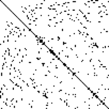
Sparsity patterns and matrix¶

Sparsity patterns are condensly viewed as monochrome matricies filled in according to 0 or non-zero.

Example: A sparsity pattern from a finite element problem in 2D.

Banded Matrices¶

Banded matrices only have non-zero elements running parallel to the main diagonal. The bandwidth describes how many parallel diagonal bands exist.

We have already seen how useful diagonal and triangular matrices are for controlling computational complexity (e.g. back-substitution).

Tridiagonal (Bandwidth 3)¶

A classic matrix structure in 1D physics problems (heat conduction, fluid flow) where every node only interacts with its immediate left and right neighbors.

n = 10
A = np.zeros((n, n))
np.fill_diagonal(A, 2)         # Main diagonal
np.fill_diagonal(A[1:], -1)    # Upper diagonal
np.fill_diagonal(A[:, 1:], -1) # Lower diagonal

print("Tridiagonal Matrix:\n", A)

plt.spy(A)
plt.title("Sparsity Pattern (Tridiagonal)")
plt.show()

Pentadiagonal (Bandwidth 5)¶

Commonly arises in 2D grid problems or higher-order finite difference methods.

n = 10
A = np.zeros((n, n))
np.fill_diagonal(A, 2)         # Main diagonal
np.fill_diagonal(A[1:], -1)    # Upper diagonal
np.fill_diagonal(A[:, 1:], -1) # Lower diagonal
np.fill_diagonal(A[4:], -2)    # Far upper diagonal
np.fill_diagonal(A[:, 4:], -1) # Far lower diagonal

plt.spy(A)
plt.title("Sparsity Pattern (Pentadiagonal)")
plt.show()

Block Matrices¶

Sometimes, a large sparse matrix can be logically partitioned into smaller sub-matrices, called blocks.

\mathbf{M} = \begin{bmatrix} 2 & -1 & 0 & | & 1 & 0 & 0 \\ -1 & 2 & -1 & | & 0 & 1 & 0 \\ 0 & -1 & 2 & | & 0 & 0 & 1 \\ --&--&--&|&--&--&-- \\ 1 & 0 & 0 & | & 2 & -1 & 0 \\ 0 & 1 & 0 & | & -1 & 2 & -1 \\ 0 & 0 & 1 & | & 0 & -1 & 2 \end{bmatrix} = \begin{bmatrix} \mathbf{A} & \mathbf{B} \\ \mathbf{C} & \mathbf{D} \end{bmatrix}

(1)

This situation arises constantly in multi-physics applications (e.g., modeling Temperature and Pressure fields simultaneously).

Instead of solving the massive matrix as a whole (monolithic solution), we can solve the blocks individually (operator splitting or segregated solving).

Solving Block Matrices¶

Because the cost of matrix inversion scales as $\mathcal{O}(n^3)$ , breaking a $2n \times 2n$ system into two $n \times n$ blocks is a massive computational savings!

For a block diagonal matrix (where off-diagonal blocks $\mathbf{B} = \mathbf{C} = \mathbf{0}$ ), the inverse is completely trivial:

\begin{bmatrix} \mathbf{A} & \mathbf{0} \\ \mathbf{0} & \mathbf{D} \end{bmatrix}^{-1} = \begin{bmatrix} \mathbf{A}^{-1} & \mathbf{0} \\ \mathbf{0} & \mathbf{D}^{-1} \end{bmatrix}

(2)