The Newton-Raphson method

import numpy as np
import plotly.graph_objects as go

try:
    import executable_engineering as exe
except ImportError:
    %pip install -q executable_engineering
    import executable_engineering as exe

The efficiency and generalizability of the Newton-Raphson method makes it the go-to root finder for nonlinear system solvers.

NB: many people abbreviate ‘The Newton-Raphson method’ to simply ‘The Newton method’, but this causes confusion with Newton’s method for optimization which is related, but a different algorithm.

The Newton-Raphson method has quadratic convergence ( $k=2$ ) near the root which is a great result! It does so, however at the cost of calculating the Jacobian and solving a linear system.

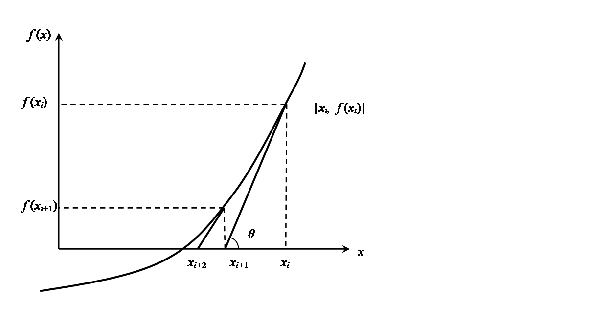
As we saw in the previous lecture, Newton’s method amounts to using the current position and the (true) tangent to estimate the next guess:

f'(x) \Delta x = - f(x)

(1)

Graphically:

Near the root, it converges quadratically, but there are some not-uncommon scenarios where it can fail.

Extensions which have greater than quadratic convergence using higher order derivative information do exist, however the additional computational cost is typically on par with another Newton-Raphson step, and therefore they are only used in certain niche applications.

The Newton-Raphson method only finds local roots, not all of them. Efficient and robust root finding requires a good initial guess.

Fortunately, in engineering, this is commonly the case!

Example of an initial guess

If we need to solve for temperature $T(x,y,z,t)$ as a nonlinear, time dependent, partial differential equation, we will be given an initial value for $T(x,y,z, t=0)$ .

When solving a nonlinear equation for $T(x,y,z,t=1)$ , what do you suppose the initial guess should be?

Answer: The initial guess should be the solution at the preceding time step!

Example: find the root of $x^3-2x+2$ ¶

There is a real root at x~-1.769.

def f(x):
  return x**3 - 2*x + 2

def df(x):
  return 3*x**2 - 2

exe.plot_newton_raphson(f, df, 2, max_iterations=8, tolerance=1e-6, title="Newton-Raphson Method", xrange=[-3, 6], yrange=[-10, 40])

Example: Find the root of $\sqrt{x}$ ¶

import warnings
warnings.filterwarnings('ignore')
def f(x):
  return np.sqrt(x)

def jacobian(x):
  return .5*x**(-1./2)

root, guesses = exe.plot_newton_raphson(f, jacobian, x0 = .1, title="Newton-Raphson Method on sqrt(x)")
print(root, guesses)

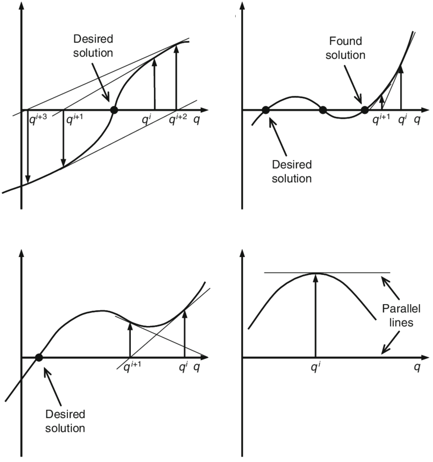
Some common failure situations¶

What went wrong in the previous example? What else could we try?

Before we talk about mitigation strategies, let’s generalize the Newton-Raphson method to N-D.

The N-D Newton-Raphson method¶

The Newton-Raphson method thus far has been described for scalar functions or scalar arguments (i.e.: 1-D).

Consider a system of $n$ unkowns $\vec{x}$ and a set of $n$ nonlinear equations that we wish to solve simultaneously:

\begin{align} f_1(\vec{x}) &= 0 \\ f_2(\vec{x}) &= 0 \\ \vdots \\ f_n(\vec{x}) &= 0 \end{align}

(2)

which may be summarized as a vector function $\vec{f}(\vec{x})=\vec{0}$ also of dimension $n$ . Since we have $n$ equations and $n$ unkowns, we can (hopefully) find an exact solution of the simultaneous set of equations, i.e.: a root.

The Newton-Raphson method generalizes quite readily except the derivative must be replaced by the vector-derivative of a vector function (called the Jacobian):

J = \frac{\partial \vec{f}}{\partial \vec{x}} = \begin{bmatrix} \frac{\partial f_1}{\partial x_1} & \frac{\partial f_1}{\partial x_2} & \dots & \frac{\partial f_1}{\partial x_n} \\ \frac{\partial f_2}{\partial x_1} & \frac{\partial f_2}{\partial x_2} & \dots & \frac{\partial f_2}{\partial x_n} \\ \vdots & \vdots & \ddots & \vdots \\ \frac{\partial f_n}{\partial x_1} & \frac{\partial f_n}{\partial x_2} & \dots & \frac{\partial f_n}{\partial x_n} \end{bmatrix}

(3)

where we can see that $J$ is a square $n \times n$ matrix. The Newton-Raphson method takes the form:

J \Delta \vec{x} = - \vec{f}

(4)

which is .... (wait for it!)... a linear system solving for the vector of increments, $\Delta\vec{x}$ !

This is an example of computational-thinking: we have broken down a muiltivariable non-linear vector function into a sequence of linear systems!

Example: solve a system of nonlinear equations¶

\begin{align} x^2 + y^2 - z &= 1 \\ x - y^2 + z^2 &= 1 \\ x y z &= 1 \end{align}

(5)

Rewrite the equations as a system of nonlinear functions:

\vec{f}(\vec{x}) = \begin{bmatrix} f_1(x, y, z) \\ f_2(x, y, z) \\ f_3(x, y, z) \end{bmatrix} = \begin{bmatrix} x^2 + y^2 - z - 1 \\ x - y^2 + z^2 -1 \\ x y z - 1 \end{bmatrix} =\vec{0}

(6)

The Jacobian is:

J = \frac{\partial \vec{f}}{\partial \vec{x}} = \begin{bmatrix} 2x & 2y & -1 \\ 1 & -2y & 2z \\ yz & xz & xy \end{bmatrix}

(7)

Now for a given $\vec{x}$ we can solve for the increment.

def f(x):
  x, y, z = x
  return np.array([
      x**2 + y**2 - z - 1,
      x - y**2 + z**2 - 1,
      x * y * z - 1
  ])

def jacobian(x):
  x, y, z = x
  return np.array([
      [2 * x, 2 * y, -1],
      [1, -2 * y, 2 * z],
      [y * z, x * z, x * y]
  ])

def newton_raphson_nd(x0, tolerance=1e-6, max_iterations=100):
  x = x0
  for iter in range(max_iterations):
    f_x = f(x)
    print("Iteration, ", iter, " the guess is ", np.round(x,3), " with residual ", np.linalg.norm(f_x) )
    J_x = jacobian(x)

    delta_x = np.linalg.solve(J_x, -f_x)
    x = x + delta_x
    if np.linalg.norm(f_x) < tolerance:
      return x
  return None

x0 = np.array([2, 2, 2])
solution = newton_raphson_nd(x0)

if solution is not None:
  print("Solution found:", solution)
else:
  print("No solution found within the maximum iterations.")

Exploring initial guesses¶

Open methods are more robust and general but compared to closed methods we loose robustness and the obvious progression towards a root (consider bracketting narrowing in).

Open methods are more succeptable to initial guess issues.

A root!¶

Let’s try a few different initial guesses to see how the method behaves.

Note something is funny with the residual...

print("\n--- Guess [3,3,3] ---")
solution1 = newton_raphson_nd(np.array([3, 3 , 3]))

Another root¶

Let’s try another initial guess.

print("\n--- Guess [10,10,10] ---")
solution2 = newton_raphson_nd(np.array([10, 10 , 10]))

Another?¶

print("\n--- Guess [-1,-1,-1] ---")
solution3 = newton_raphson_nd(np.array([-1, -1 ,-1]))

And another?¶

Note what’s happening to guesses and the residual... odd behaviour indeed!

print("\n--- Guess [-10,0,-10] ---")
solution4 = newton_raphson_nd(np.array([-10, 0,-10]))

Example: find the root of x3−2x+2x^3-2x+2x3−2x+2¶

Example: Find the root of x\sqrt{x}x​¶