import numpy as np
import sympy as sp
import plotly.graph_objects as go

try:
    import executable_engineering as exe
except ImportError:
    %pip install -q executable_engineering
    import executable_engineering as exe
Optimal Evaluation Nodes: The Gauss Points
Up until this point, we have been using techniques for which the data points are fixed, (hopefully) evenly spaced, and at the limits of our subdomains.
Gaussian quadrature assumes you are free to choose the evaluation points . The goal is then to find special sets of points (called Gauss points) and weights for which the integral is computed with maximal polynomial degree precision.
The 2-Point Gauss-Legendre Formula
Let’'s propose a formula for the integral of a function in the range :
where the unknowns are (4 degrees of freedom). We require this formula to integrate monomials exactly:
Solving this system yields:
That is a remarkable result! Any cubic polynomial can be integrated exactly merely through the sum of the function evaluated at two points!
def two_point_gaussian_quadrature(f):
    return f(-1.0 / np.sqrt(3)) + f(1.0 / np.sqrt(3))

x = sp.var("x")

def quad_tester(expr):
    fcn = sp.lambdify(x, expr, modules=["numpy"])
    fI = float(sp.integrate(expr, (x, -1, 1)))
    num_val = float(two_point_gaussian_quadrature(fcn))
    print(f"Function: {expr} | Exact: {fI:.6f} | Error: {num_val - fI:.2e}")

quad_tester(x**2)
quad_tester(x**3 - x**2 + sp.pi * x + 17)
quad_tester(-10**9 * x**3 + sp.exp(1) * x**2 - sp.sqrt(sp.pi) * x + 42)
Transformation to an Arbitrary Domain 
The preceding case specified integration limits on . To apply Gaussian quadrature to arbitrary integration limits , we perform a coordinate change:
where .
def flex_gq(f, a, b):
    x0 = -1.0 / np.sqrt(3)
    x1 = 1.0 / np.sqrt(3)
    x_d0 = ((b + a) + (b - a) * x0) / 2.0
    x_d1 = ((b + a) + (b - a) * x1) / 2.0
    dx = (b - a) / 2.0
    return (f(x_d0) + f(x_d1)) * dx

def flex_gq_tester(expr, a, b):
    fcn = sp.lambdify(x, expr, modules=["numpy"])
    exact = float(sp.integrate(expr, (x, a, b)))
    approx = float(flex_gq(fcn, a, b))
    print(f"Integral of {expr} on [{a}, {b}]: Exact = {exact:.6f}, Approx = {approx:.6f}, Error = {approx - exact:.2e}")

flex_gq_tester(x**2, 0, 1)
flex_gq_tester(x**3 - x**2 + sp.pi * x + 17, 0, 1)
The -point Gauss-Legendre Formula
Jinkies!
The method may be generalized to -point quadrature that integrates polynomials up to degree exactly:
with given by Legendre polynomial weights:
| Integration order | Coefficient () | Gauss Point () | Error Term |
|---|---|---|---|
| 2 | |||
| 3 | |||
| 4 | |||
| 5 |
Error Analysis for Gauss-Legendre Quadrature
Note that the error is given in terms of higher derivatives of , since the step size is no longer an issue. In general, the error is:
for some .
Multidimensional Gauss-Legendre Quadrature
Due to the separable nature of multidimensional integration, extending this concept to dimensions is an exercise in repeated application:
Quadrilateral Elements
An example of a quadrilateral with a 3rd integration order is shown below, illustrating the mapping between computational parent coordinates (left) and real physical coordinates (right):
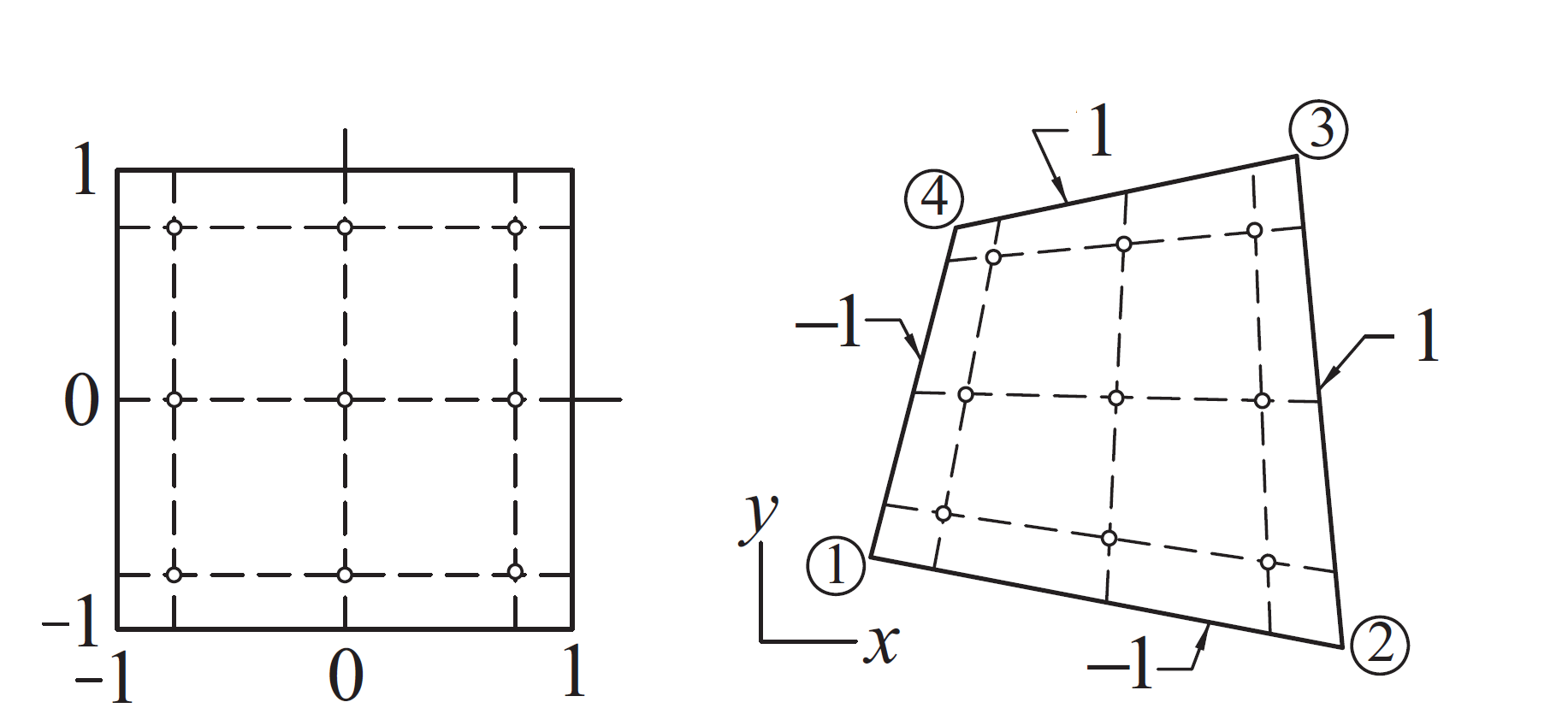
Coordinates in physical space are interpolated using bilinear shape functions :
with bilinear shape functions:
Triangular Elements and Area Coordinates
In irregular domains, a quadrilateral may reduce a side length to zero, thereby becoming a degenerate quadrilateral, or simply a triangle.
Consider dividing a triangle into 3 sub-areas by connecting the vertices to an interior point :
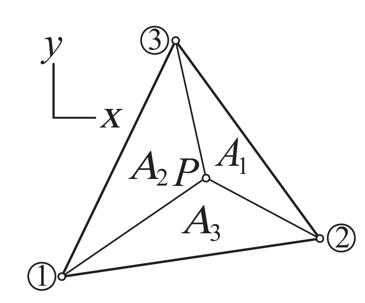
so as to define areas . The area coordinates of are:
and since :
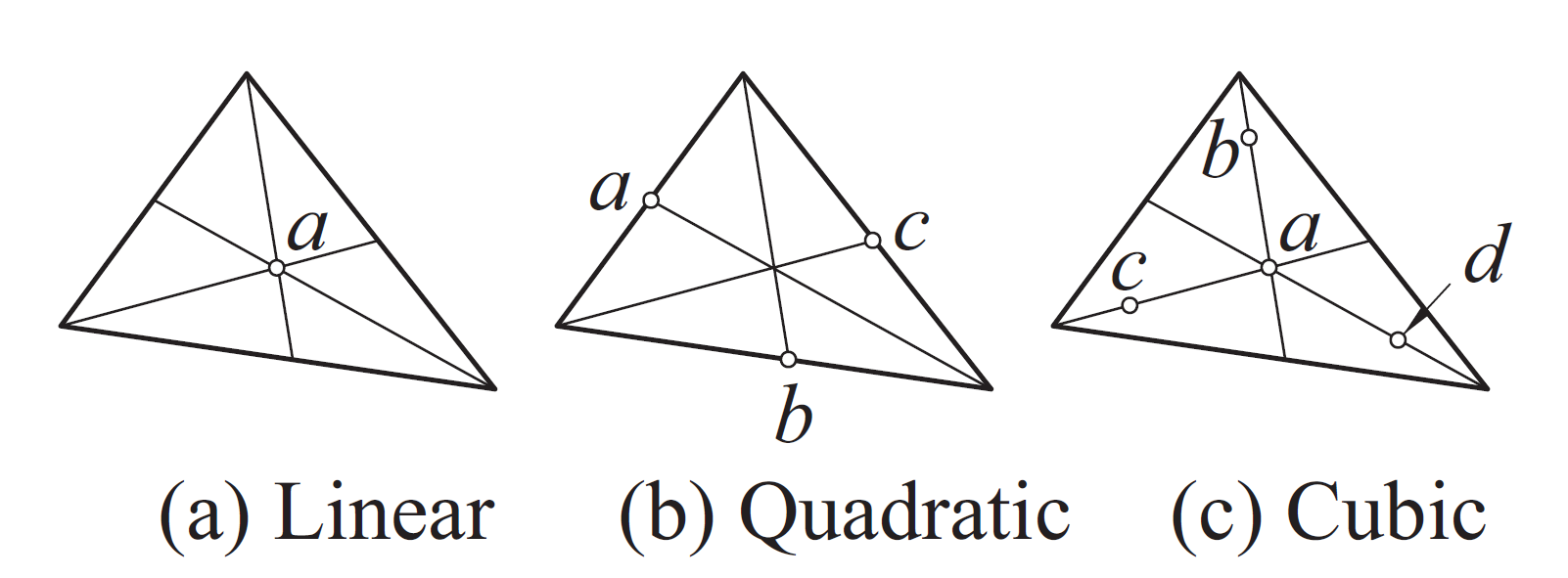
Gauss integration points on triangular elements are specified in these normalized area coordinates: