Numerical integration - Executable Engineering: Interactive Numerical Methods in Python

import numpy as np
import plotly.graph_objects as go

try:
    import executable_engineering as exe
except ImportError:
    %pip install -q executable_engineering
    import executable_engineering as exe

Motivation for Numerical Quadrature¶

Numerical integration approximates analytic integration, and is particularly useful because:

Analytic integrals may be hard to find if they exist at all.
Functions may only be known at a set of discrete sample points.

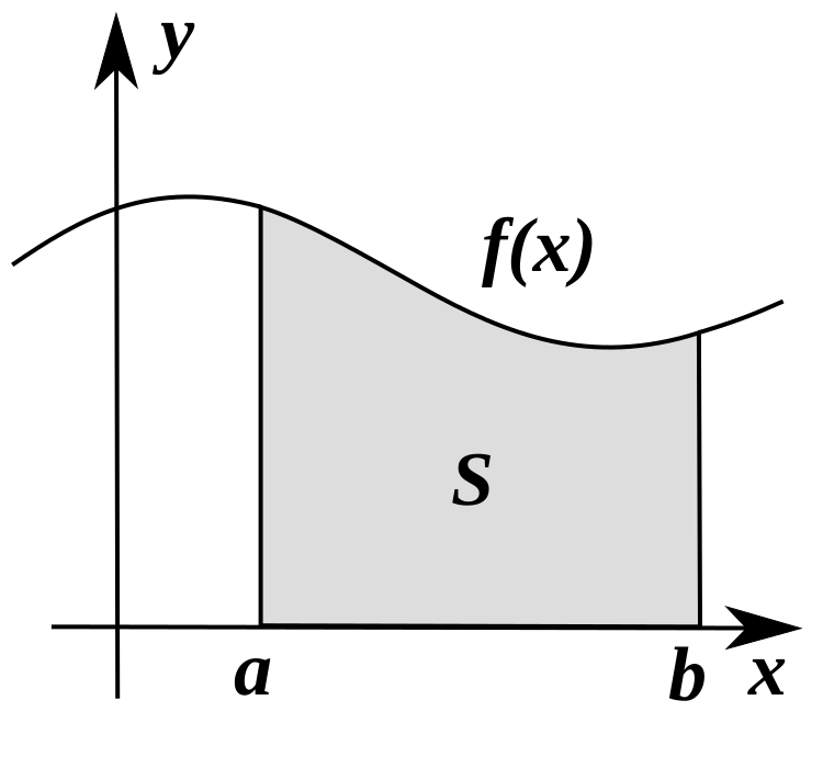
For definite integrals (i.e. with finite limits), numerical integration is called numerical quadrature.

Aside: The integral sign $\int$ looks like an elongated ‘S’ because summa (Latin for summation) is exactly what we are doing!

Continuous Functions vs. Discrete Datasets¶

The methods discussed in this chapter consider two primary engineering cases:

Discrete dataset $(x_i, f_i)$ is given: The values are fixed by experiment or observation, requiring panel-based interpolation (e.g. Newton-Cotes rules).
Callable function $f(x)$ is available: The integrand can be sampled at any arbitrary evaluation point, enabling adaptive node placement (Romberg rule, Gauss-Legendre quadrature).