Gradient-free optimizers - Executable Engineering: Interactive Numerical Methods in Python

When an objective function $f(\mathbf{x})$ is non-differentiable, noisy, or computationally expensive to differentiate, gradient-free (direct search) methods provide robust optimization using only function evaluations.

We explore two classical direct-search methods:

Powell’s method (conjugate direction search via 1D line searches)
Nelder-Mead downhill simplex (heuristic geometric deformation / amoeba method)

import numpy as np
import scipy.optimize as optimize
import plotly.graph_objects as go

try:
    import executable_engineering as exe
except ImportError:
    %pip install -q executable_engineering
    import executable_engineering as exe

from executable_engineering import plot_optimization_path_3d

Powell’s method¶

Powell’s method uses a starting point and an initial set of direction vectors (typically the coordinate axes). The function is minimized sequentially along each direction using 1D line searches.

Subsequent direction vectors are obtained through an important geometric observation:

The line connecting the minima of parallel line searches on quadratic functions passes directly through the minimum.

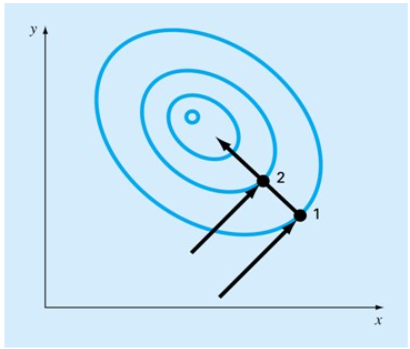
Powell showed that this procedure generates conjugate directions without requiring any derivative information. Near a minimum, where the objective behaves quadratically, this achieves fast quadratic-like convergence!

The Powell algorithm¶

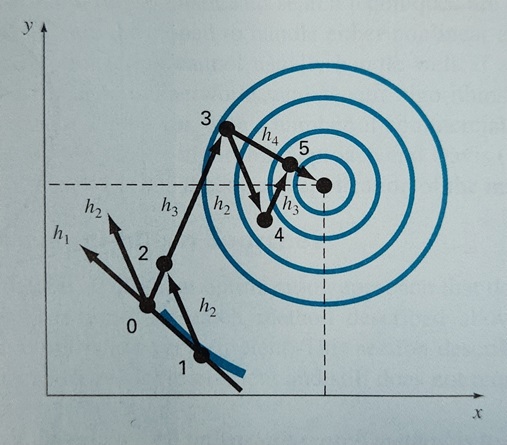
The algorithm proceeds as follows (from Chapra and Canale - Numerical Methods for Engineers):

Start at 0 with directions $\mathbf{h}_1$ and $\mathbf{h}_2$ .
Search from 0 along $\mathbf{h}_1$ to find minimum 1.
Search from 1 along $\mathbf{h}_2$ to find minimum 2.
Define new direction $\mathbf{h}_3$ connecting 0 to 2.
Search from 2 along $\mathbf{h}_3$ to find minimum 3.
From 3, search along $\mathbf{h}_2$ to find 4.
From 4, search along $\mathbf{h}_3$ to find 5.
Use points 5 and 3 to define $\mathbf{h}_4$ .
$\mathbf{h}_3$ and $\mathbf{h}_4$ are conjugate; the exact minimum of a quadratic can now be reached directly!

Example: 2D optimization with Powell’s method¶

Minimize the 2D Rosenbrock ‘banana’ function:

f(x_1, x_2) = (1 - x_1)^2 + 100 (x_2 - x_1^2)^2

(1)

The function has a curved, narrow parabolic valley with a global minimum at $(1, 1)$ where $f(1, 1) = 0$ .

def rosenbrock(x):
    return (1 - x[0])**2 + 100 * (x[1] - x[0]**2)**2

x0 = np.array([-1.0, 2.5])
result = optimize.minimize(rosenbrock, x0, method='Powell', options={'return_all': True})
print("Minimum found at x =", result.x)
print("Minimum function value =", result.fun)

plot_optimization_path_3d(rosenbrock, result.allvecs, x_range=(-2, 2), y_range=(-1, 3), title="Powell's Method on Rosenbrock Function")

Nelder-Mead downhill simplex (amoeba method)¶

The Nelder-Mead method works by moving an N-D simplex downhill until it surrounds a minimum, then contracts until a specified threshold is reached.

A simplex is the simplest geometric figure with $N+1$ vertices in $N$ dimensions (a triangle in 2D, a tetrahedron in 3D).

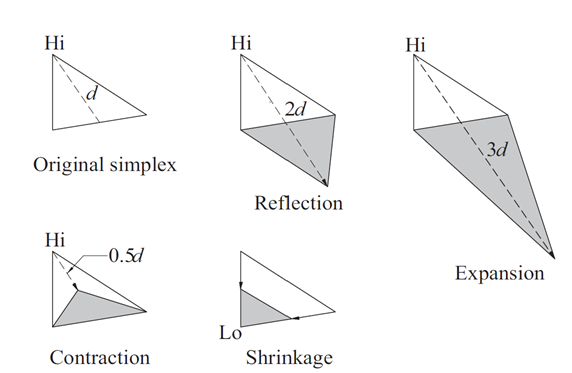
The algorithm proceeds by identifying the ‘Hi’ ( $x_h$ , worst) and ‘Lo’ ( $x_l$ , best) vertices:

Reflection: Move ‘Hi’ through the opposite face, preserving the volume of the simplex.
Expansion: Move ‘Hi’ further to increase the simplex volume in a promising direction.
Contraction: Move ‘Hi’ a fraction towards the opposite face when reflection overshoots.
Shrinkage: Move all vertices toward ‘Lo’ if no step improves the objective.

Nelder-Mead algorithm¶

Decision logic:

Try reflection.
if new vertex <= old Lo: accept reflection
  Try expansion.
  if new vertex <= old Lo: accept expansion.
else:
  if new vertex > old Hi:
    Try contraction.
    if new vertex <= old Hi: accept contraction.
  else: use shrinkage.

Known as the ‘Amoeba method’ because the simplex deforms and crawls like a single-celled organism across the energy landscape. While requiring more evaluations than gradient methods, it is exceptionally robust for noisy or discontinuous functions.

Example: Nelder-Mead on the Rosenbrock function¶

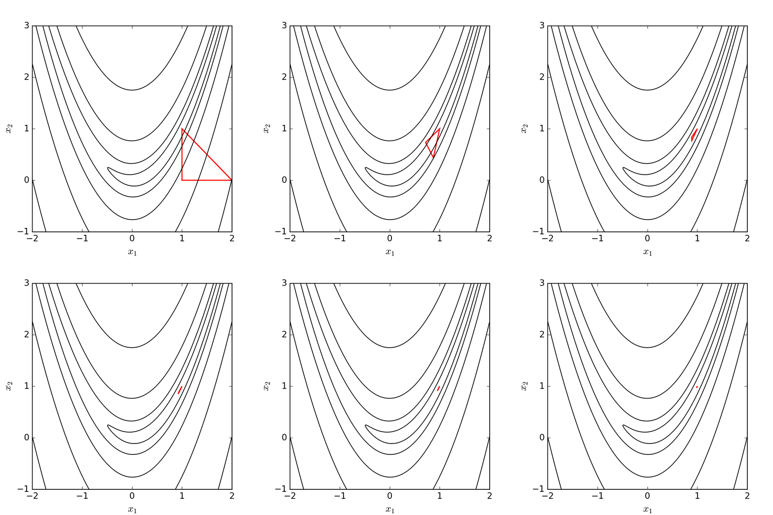
Watch the simplex crawl through the narrow banana valley toward $(1, 1)$ :

x0 = np.array([-1.0, 2.5])
result = optimize.minimize(rosenbrock, x0, method='Nelder-Mead', options={'return_all': True})
print("Minimum found at x =", result.x)
print("Minimum function value =", result.fun)

plot_optimization_path_3d(rosenbrock, result.allvecs, x_range=(-2, 2), y_range=(-1, 3), title="Nelder-Mead on Rosenbrock Function")

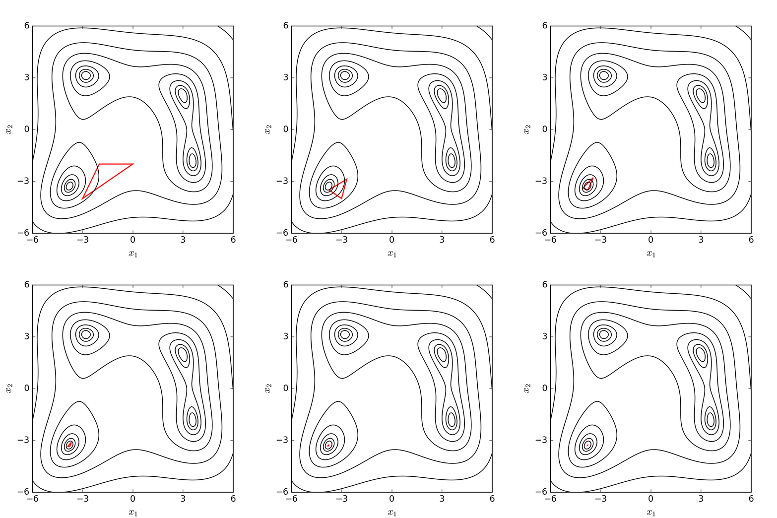
Example: Nelder-Mead on the Himmelblau function¶

Himmelblau’s function has four identical global minima where $f(x_1, x_2) = 0$ :

f(x_1, x_2) = (x_1^2 + x_2 - 11)^2 + (x_1 + x_2^2 - 7)^2

(2)

def himmelblau(x):
    return (x[0]**2 + x[1] - 11)**2 + (x[0] + x[1]**2 - 7)**2

x0 = np.array([-0.5, -0.5])
result = optimize.minimize(himmelblau, x0, method='Nelder-Mead', options={'return_all': True})
print("Minimum found at x =", result.x)
print("Minimum function value =", result.fun)

plot_optimization_path_3d(himmelblau, result.allvecs, x_range=(-6, 6), y_range=(-6, 6), title="Nelder-Mead on Himmelblau Function")