Second order derivatives - Executable Engineering: Interactive Numerical Methods in Python

import numpy as np
import plotly.graph_objects as go

try:
    import executable_engineering as exe
except ImportError:
    %pip install -q executable_engineering
    import executable_engineering as exe

# Setup rocket velocity and analytical acceleration from earlier lessons
def v(t):
    return 2000 * np.log((14 * 10**4) / (14 * 10**4 - 2100 * t)) - 9.8 * t

def a(t):
    return (42 * 10**5) / (14 * 10**4 - 2100 * t) - 9.8

def forward_difference(f, x, h):
    return (f(x + h) - f(x)) / h

def central_difference(f, x, h):
    return (f(x + h) - f(x - h)) / (2 * h)

t = np.linspace(0, 30, 100)
a_fd_h2 = forward_difference(v, t, h=2)
a_cd_h2 = central_difference(v, t, h=2)

Forward Difference (Second Order)¶

We can similarly derive higher order derivatives in forward, backward, and central approximations. Once obtained, we can also use the second order derivative to improve our estimate of the first order derivative.

Consider the Taylor expansions:

\begin{aligned} f(x+2h) &= f(x)+ 2 f'(x) h + f''(x)\frac{4 h^2}{2} + O(h^3) \\ f(x+h) &= f(x)+ f'(x) h + f''(x)\frac{h^2}{2} + O(h^3) \end{aligned}

(1)

Multiplying the second equation by 2 and subtracting from the first eliminates the first derivative term:

f''(x) = \frac{f(x+2h) - 2 f(x+h) + f(x)}{h^2} + O(h)

(2)

def second_forward_difference(f, x, h):
    return (f(x + 2 * h) - 2 * f(x + h) + f(x)) / (h**2)

Alternative Derivation¶

Note we could also arrive at this considering the 1st derivative of the 1st derivatives:

\begin{aligned} f'(x) &= \frac{f(x+h) - f(x)}{h} \\ f'(x+h) &= \frac{f(x+2h) - f(x+h)}{h} \\ f''(x) &= \frac{f'(x+h) - f'(x)}{h} = \frac{f(x+2h) - 2f(x+h) + f(x)}{h^2} \end{aligned}

(3)

which lends itself directly to a recursive implementation.

A More Accurate First Derivative¶

We can now revisit the approximation of $f'(x)$ and use our approximation of $f''(x)$ to improve it!

Recall the Taylor series:

f(x+h) = f(x) + f'(x)h + f''(x)\frac{h^2}{2} + O(h^3)

(4)

Substituting our $f''(x)$ forward approximation yields:

f'(x) = \frac{-f(x+2h) + 4f(x+h) - 3f(x)}{2h} + O(h^2)

(5)

This is a nice result, but notice that we now need three function calls to achieve the same accuracy as the central difference (which only needs two function calls).

The general formula for $n$ -th order forward derivatives is:

f^{(n)}(x) = \sum_{i=0}^n (-1)^{n-i} \binom{n}{i} f(x+ih)

(6)

which one could use to successively build higher and higher order algorithms.

Example: Error Comparison for Improved Forward Difference¶

Compare the error for the improved forward difference method against standard forward difference and central difference:

def forward_difference_2(f, x, h):
    return (-f(x + 2 * h) + 4 * f(x + h) - 3 * f(x)) / (2 * h)

a_fd2_h2 = forward_difference_2(v, t, h=2)
a_fd2_h1 = forward_difference_2(v, t, h=1)

np.stack([a_fd_h2 - a(t), a_fd2_h2 - a(t), a_fd2_h1 - a(t), a_cd_h2 - a(t)]).T[1:5, :]

Backward Difference (Second Order)¶

Following a similar derivation, the backward second derivative is:

f''(x) = \frac{f(x) - 2 f(x-h) + f(x-2h)}{h^2} + O(h)

(7)

and the second-order accurate backward first derivative is:

f'(x) = \frac{3 f(x) - 4 f(x-h) + f(x-2h)}{2h} + O(h^2)

(8)

def backward_difference_2(f, x, h):
    return (3 * f(x) - 4 * f(x - h) + f(x - 2 * h)) / (2 * h)

a_bd2_h2 = backward_difference_2(v, t, h=2)
print("Second-order backward difference error (first 4 steps):")
print((a_bd2_h2 - a(t))[2:6])

Central Difference (Second Order)¶

Finally, simply adding the forward and backward Taylor expansions gives the central difference for the second derivative:

\begin{aligned} f(x+h) &= f(x) + f'(x) h + f''(x) \frac{h^2}{2} + f'''(x)\frac{h^3}{6} + f^{(4)}(x)\frac{h^4}{24} + O(h^5) \\ f(x-h) &= f(x) - f'(x) h + f''(x) \frac{h^2}{2} - f'''(x)\frac{h^3}{6} + f^{(4)}(x)\frac{h^4}{24} + O(h^5) \end{aligned}

(9)

Adding the two expressions cancels all odd powers of $h$ :

f(x+h) + f(x-h) = 2 f(x) + f''(x) h^2 + O(h^4)

(10)

Rearranging for $f''(x)$ yields:

f''(x) = \frac{f(x+h) - 2 f(x) + f(x-h)}{h^2} + O(h^2)

(11)

which is second-order accurate!

def central_difference_2(f, x, h):
    return (f(x + h) - 2 * f(x) + f(x - h)) / (h**2)

Summary of Finite Difference Algorithms¶

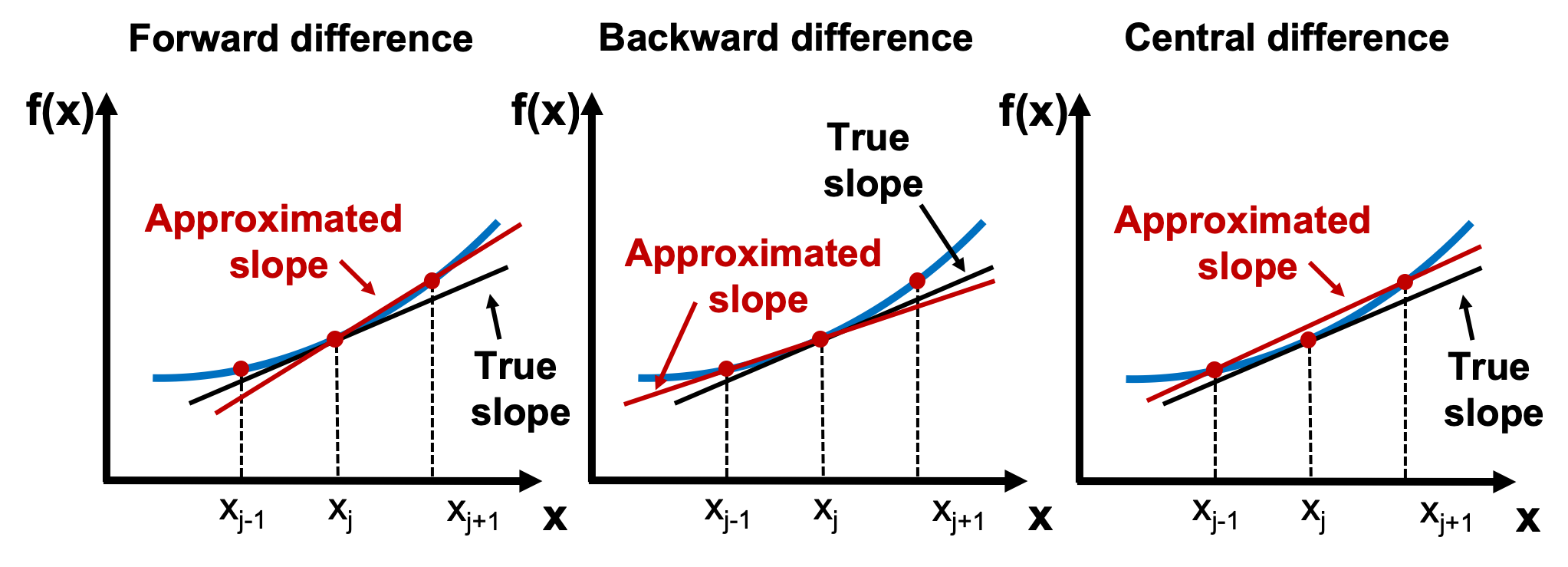
Summary Table of Finite Difference Stencils

The accuracy of the approximation can be improved in two ways:

Decrease step size ( $h \to 0$ ).
Use approximated higher order derivatives to correct lower order ones.

Central difference yields the same order of accuracy as the improved forward/backward difference with one fewer function evaluation, but requires points on both sides of the evaluation point.