Simpson’s rules

import numpy as np
import scipy as sp
import plotly.graph_objects as go

try:
    import executable_engineering as exe
except ImportError:
    %pip install -q executable_engineering
    import executable_engineering as exe

Simpson’s 1/3 Rule¶

Continuing our polynomial degrees, we arrive at the Newton-Cotes order 2 method with a quadratic. Now we need 3 data points per fit, which we can envision as a parabola spanning two intervals:

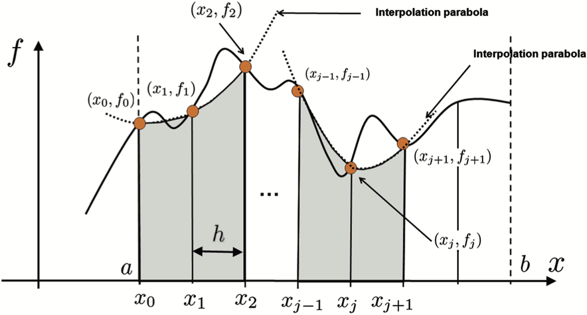
We can fit a quadratic with Lagrange polynomials with $x_i-x_{i-1} = x_{i+1}-x_i = h$ :

f(x) \approx \frac{f(x_{i-1})}{2h^2} (x - x_i)(x - x_{i+1}) - \frac{f(x_i)}{h^2} (x - x_{i-1})(x - x_{i+1}) + \frac{f(x_{i+1})}{2h^2} (x - x_{i-1})(x - x_i)

(1)

Integrating this quadratic over $[x_{i-1}, x_{i+1}]$ yields:

\int_{x_{i-1}}^{x_{i+1}} f(x) \,\mathrm{d}x = \frac{h}{3} [f(x_{i-1}) + 4 f(x_i) + f(x_{i+1})] + O(h^5)

(2)

numerical_integration_module.py

1
2
3
4
5
6
7
8
9
10
11
12
13
14
15
16
17
18
19
20
21
22
23
24
25
def simpsons_13(f, a, b, n):
    if n <= 0 or n % 2 != 0:
        raise ValueError("Simpson's 1/3 Rule requires a positive even number of subintervals.")

    h = (b - a) / n
    x_points = np.linspace(a, b, n + 1)
    y_points = np.asarray(f(x_points))

    integral_approx = (h / 3) * (
        y_points[0]
        + y_points[-1]
        + 4 * np.sum(y_points[1:-1:2])
        + 2 * np.sum(y_points[2:-1:2])
    )

    return {
        "x_points": x_points,
        "y_points": y_points,
        "n": n,
        "integral_approx": integral_approx,
        "a": a,
        "b": b,
        "h": h,
    }

exe.display_source(exe.simpsons_13)

result = exe.simpsons_13(np.sin, a=0, b=np.pi, n=4)
fig = exe.visualize_simpsons_13(np.sin, result)
fig.show()

Error Analysis: Simpson’s 1/3 Rule¶

For the error, take the Taylor series approximation of $f(x)$ around $x_i$ :

f(x) = f(x_i) + f'(x_i)(x - x_i) + \frac{f''(x_i)}{2}(x-x_i)^2 + \frac{f'''(x_i)}{6}(x-x_i)^3 + \frac{f^{(4)}(x_i)}{24}(x-x_i)^4 + O(h^5)

(3)

Because the interval $[-h, h]$ is symmetric around $x_i$ , odd-degree terms integrate to zero!

The local error is:

E_{local} = -\frac{f^{(4)}(x_i)}{90} h^5

(4)

For $n$ subdivisions, the composite error scales as $n \cdot O(h^5) = O(h^4)$ , achieving fourth-order convergence!

Example: Convergence Comparison¶

Integrate $\sin(x)$ on $[0, \pi]$ (exact value = 2) with Simpson’'s 1/3 Rule and compare to the midpoint and trapezoid rules:

a = 0
b = np.pi

for n in [2, 4, 8, 16, 32]:
    trapezoid_result = exe.trapezoid_rule(np.sin, a, b, n)['integral_approx']
    midpoint_result = exe.midpoint_riemann(np.sin, a, b, n)['integral_approx']
    simps_result = exe.simpsons_13(np.sin, a, b, n)['integral_approx']
    print(f"n = {n:2d}: Trapezoid err = {abs(trapezoid_result - 2):.6e}, Midpoint err = {abs(midpoint_result - 2):.6e}, Simpson err = {abs(simps_result - 2):.6e}")

Simpson’s 3/8 Rule (Order 3)¶

Yowza! Notice the rapid convergence of Simpson’s rule!

The final polynomial we will discuss is a cubic fit to 4 data points (3 intervals). This results in:

\int_{x_i}^{x_{i+3}} f(x) \,\mathrm{d}x = \frac{3}{8}h [f(x_i) + 3f(x_{i+1}) + 3f(x_{i+2}) + f(x_{i+3})] + O(h^5)

(5)

Note the $3/8$ which lends its name. This rule takes 3 intervals, and therefore a combination of the $1/3$ and $3/8$ rules covers all possibilities (even or odd number of intervals) without loss of error order.

Note that the composite order of error is the same as the $1/3$ rule ( $O(h^4)$ ).

numerical_integration_module.py

1
2
3
4
5
6
7
8
9
10
11
12
13
14
15
16
17
18
19
20
21
22
23
24
25
def simpsons_38(f, a, b, n):
    if n <= 0 or n % 3 != 0:
        raise ValueError("Simpson's 3/8 Rule requires a positive number of subintervals divisible by 3.")

    h = (b - a) / n
    x_points = np.linspace(a, b, n + 1)
    y_points = np.asarray(f(x_points))

    weights = np.full(n + 1, 3.0)
    weights[0] = 1
    weights[-1] = 1
    weights[3:-1:3] = 2

    integral_approx = (3 * h / 8) * np.sum(weights * y_points)

    return {
        "x_points": x_points,
        "y_points": y_points,
        "n": n,
        "integral_approx": integral_approx,
        "a": a,
        "b": b,
        "h": h,
    }

exe.display_source(exe.simpsons_38)

result = exe.simpsons_38(np.sin, a=0, b=np.pi, n=6)
fig = exe.visualize_simpsons_38(np.sin, result)
fig.show()

Package Implementation: SciPy’s `simpson`¶

In practice, scipy.integrate.simpson provides a robust composite Simpson’s rule implementation for discrete arrays that automatically handles both even and odd numbers of intervals.

x = np.linspace(0, np.pi, 9)  # 8 intervals
y = np.sin(x)

scipy_result = sp.integrate.simpson(y, x=x)
print(f"SciPy Simpson result: {scipy_result:.6f} (Error: {abs(scipy_result - 2):.6e})")

Simpson’s 1/3 Rule¶

Error Analysis: Simpson’s 1/3 Rule¶

Example: Convergence Comparison¶

Simpson’s 3/8 Rule (Order 3)¶

Package Implementation: SciPy’s simpson¶

Package Implementation: SciPy’s `simpson`¶