Trapezoid rule - Executable Engineering: Interactive Numerical Methods in Python

import numpy as np
import plotly.graph_objects as go

try:
    import executable_engineering as exe
except ImportError:
    %pip install -q executable_engineering
    import executable_engineering as exe

Derivation of the Trapezoid Rule¶

The next polynomial degree is 1; a line.

Given the points $x_i$ , $x_{i+1}$ , $f_i$ , and $f_{i+1}$ :

f(x) \approx f_i + \frac{f_{i+1} - f_i}{x_{i+1} - x_i}(x - x_i)

(1)

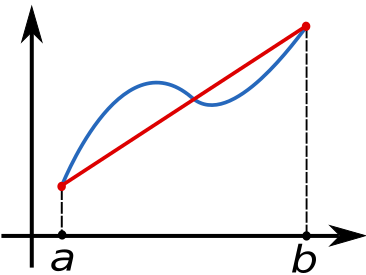
Integrating this linear interpolant over $[x_i, x_{i+1}]$ with step $h = x_{i+1} - x_i$ :

\int_{x_i}^{x_{i+1}} f(x) \,\mathrm{d}x \approx \frac{h}{2} [f_i + f_{i+1}]

(2)

Summing over all $n$ subdivisions yields the composite trapezoid rule:

\int_a^b f(x) \,\mathrm{d}x \approx \frac{h}{2} \left[f(a) + 2 \sum_{i=1}^{n-1} f(x_i) + f(b)\right]

(3)

numerical_integration_module.py

1
2
3
4
5
6
7
8
9
10
11
12
13
14
15
16
17
18
19
def trapezoid_rule(f, a, b, n):
    h = (b - a) / n
    x_points = np.linspace(a, b, n + 1)
    y_points = f(x_points)

    widths = np.diff(x_points)
    integral_approx = np.sum(widths * (y_points[:-1] + y_points[1:]) / 2)

    return {
        "x_points": x_points,
        "y_points": y_points,
        "widths": widths,
        "n": n,
        "integral_approx": integral_approx,
        "a": a,
        "b": b,
        "h": h,
    }

exe.display_source(exe.trapezoid_rule)

result = exe.trapezoid_rule(np.sin, a=0, b=np.pi, n=5)
fig = exe.visualize_trapezoid_rule(np.sin, result)
fig.show()

Loading...

Error Analysis of the Trapezoid Rule¶

The accuracy is calculated from the Taylor series expansion of $f(x)$ around the midpoint $y_i = \frac{x_{i+1} + x_i}{2}$ :

\begin{aligned} f(x) &= f(y_i) + f'(y_i)(x - y_i) + \frac{f''(y_i)}{2}(x - y_i)^2 + O(h^3) \\ \int_{x_i}^{x_{i+1}} f(x) \,\mathrm{d}x &= f(y_i) h + \frac{f''(y_i)}{24} h^3 + O(h^5) \end{aligned}

(4)

Meanwhile, evaluating the trapezoid approximation with the same expansion gives:

\frac{h}{2}[f(x_i) + f(x_{i+1})] = f(y_i) h + \frac{f''(y_i)}{8} h^3 + O(h^5)

(5)

The difference yields the local truncation error:

E_{local} = -\frac{f''(y_i)}{12} h^3

(6)

Summing over all $n = (b-a)/h$ elements gives a composite error of $O(h^2)$ , confirming second-order convergence!

Example: Comparing Trapezoid and Midpoint Methods¶

Integrate $\sin(x)$ from 0 to $\pi$ (exact analytical value = 2) with the midpoint and trapezoid rules across increasing resolutions:

a = 0
b = np.pi

for n in [2, 4, 8, 16, 32]:
    trapezoid_result = exe.trapezoid_rule(np.sin, a, b, n)
    midpoint_result = exe.midpoint_riemann(np.sin, a, b, n)
    print(f"n = {n:2d}: Trapezoid error = {abs(trapezoid_result['integral_approx'] - 2):.6f}, Midpoint error = {abs(midpoint_result['integral_approx'] - 2):.6f}")

n =  2: Trapezoid error = 0.429204, Midpoint error = 0.221441
n =  4: Trapezoid error = 0.103881, Midpoint error = 0.052344
n =  8: Trapezoid error = 0.025768, Midpoint error = 0.012909
n = 16: Trapezoid error = 0.006430, Midpoint error = 0.003216
n = 32: Trapezoid error = 0.001607, Midpoint error = 0.000803

Observations: Midpoint vs. Trapezoid¶

Notice we get quadratic convergence ( $O(h^2)$ ) for both methods, but the midpoint method is actually twice as accurate for the same number of intervals!

However, the midpoint rule requires evaluation at interior points $y_i$ , which are not available when working with fixed discrete datasets. The trapezoid rule, by contrast, operates directly on endpoint samples!