Reimann’s integrals

Reimann’s integral is the simplest of the Newton-Cotes formulae with a polynomial of degree \(0\), i.e. a constant over each subdivision. Variants exist for taking the function value at the left limit, middle, or right.

Left and right Reimann integrals

If we take the function value at the left of the subdomain \([x_i, x_{i+1}]\) , we obtain the left Reimann integral,

\[\int_a^b f(x) dx \approx \sum_{i = 0}^{n-1} hf(x_i),\]

or using the right limit,

\[\int_a^b f(x) dx \approx \sum_{i = 0}^{n-1} hf(x_{i+1}) = \sum_{i = 1}^{n} hf(x_i),\]

These correspond to taking the function values on the left and right of the subdivision as the constant over the entire interval:

import numpy as np
import matplotlib.pyplot as plt

def f(x):
  """The function to integrate."""
  return x**2

def left_reimann(f, a, b, n):
  """Calculates the left Riemann sum."""
  dx = (b - a) / n
  x_values = np.linspace(a, b - dx, n)
  return np.sum(f(x_values) * dx)

def right_reimann(f, a, b, n):
  """Calculates the right Riemann sum."""
  dx = (b - a) / n
  x_values = np.linspace(a + dx, b, n)
  return np.sum(f(x_values) * dx)

# Integration interval
a = 0
b = 10
# Number of subdivisions
n = 10

# Calculate left and right Riemann sums
left_sum = left_reimann(f, a, b, n)
right_sum = right_reimann(f, a, b, n)

# Generate x and y values for the function
x_values = np.linspace(a, b, 100)
y_values = f(x_values)

# Create the left Riemann sum figure
plt.figure(figsize=(12, 6))
plt.subplot(1, 2, 1)
plt.plot(x_values, y_values, label='f(x)')
dx = (b - a) / n
x_rect = np.linspace(a, b - dx, n)
for i in range(n):
  plt.bar(x_rect[i], f(x_rect[i]), width=dx, alpha=0.5, align='edge', color='blue')
plt.title('Left Riemann Sum')
plt.xlabel('x')
plt.ylabel('f(x)')
plt.scatter(x_rect, f(x_rect), color='red', label='Left Riemann Points')
plt.grid(True)  # Turn on the grid
plt.legend()

# Create the right Riemann sum figure
plt.subplot(1, 2, 2)
plt.plot(x_values, y_values, label='f(x)')
x_rect = np.linspace(a + dx, b, n)
for i in range(n):
  plt.bar(x_rect[i]-dx, f(x_rect[i]), width=dx, alpha=0.5, align='edge', color='green')
plt.title('Right Riemann Sum')
plt.xlabel('x')
plt.ylabel('f(x)')
plt.scatter(x_rect, f(x_rect), color='red', label='Right Riemann Points')
plt.grid(True)  # Turn on the grid
plt.legend()

plt.tight_layout()
plt.show()

print("True integral, 1/3 x^3 = 333. Left integral, ", left_sum, "Right integral, ", right_sum)

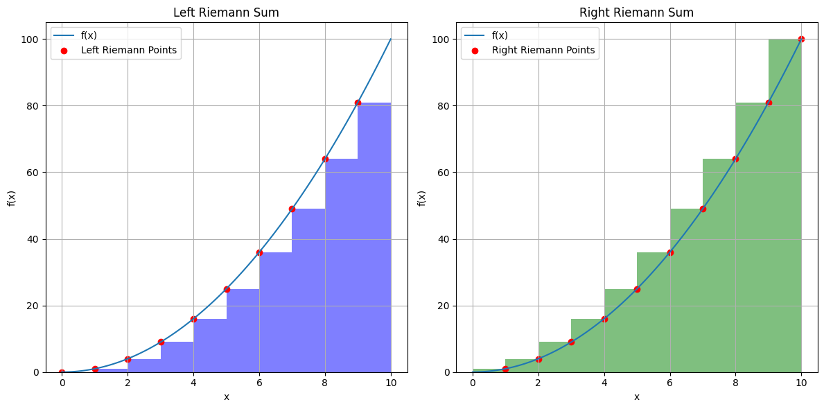
True integral, 1/3 x^3 = 333. Left integral,  285.0 Right integral,  385.0

Error

To analyse the error, consider integrating the Taylor expansion of the left integral (the right being trivially similar),

\[\begin{split} \begin{align} f(x) &= f(x_i) + f^{\prime}(x_i)(x-x_i) + \cdots \\ \int_{x_i}^{x_{i+1}} f(x) dx &= \int_{x_i}^{x_{i+1}} (f(x_i) + f^{\prime}(x_i)(x-x_i) + \cdots)\ dx \\ &= \int_{x_i}^{x_{i+1}} f(x_i) dx + \int_{x_i}^{x_{i+1}} f^{\prime}(x_i)(x-x_i)dx + \cdots.\ \end{align}\end{split}\]

since the integral distributes. Integrating term by term we get,

\[\begin{split} \begin{align} \int_{x_i}^{x_{i+1}} f(x) dx &= hf(x_i) + \frac{h^2}{2}f^{\prime}(x_i) + O(h^3), \\ &= hf(x_i) + O(h^2)\end{align} \end{split}\]

For each subinterval, the left integral is \(O(h^2)\).

If we sum the \(O(h^2)\) error over the entire Riemann sum, we get \(nO(h^2)\). The relationship between \(n\) and \(h\) is

\[h = \frac{b - a}{n},\]

and so our total error becomes \(\frac{b - a}{h}O(h^2) = O(h)\) over the whole interval. Thus the overall accuracy is \(O(h)\).

The Midpoint Reimann integral

Rather than favour the left or right subdomain limit, let’s take hte midpoint \(y_i = \frac{x_{i+1} + x_i}{2}\). The Midpoint Rule says

\[\int_a^b f(x)dx \approx \sum_{i = 0}^{n-1} hf(y_i).\]

import numpy as np
import matplotlib.pyplot as plt

def f(x):
  """The function to integrate."""
  return x**2

def midpoint_reimann(f, a, b, n):
  """Calculates the midpoint Riemann sum."""
  dx = (b - a) / n
  x_values = np.linspace(a + dx / 2, b - dx / 2, n)
  return np.sum(f(x_values) * dx)


# Integration interval
a = 0
b = 10
# Number of subdivisions
n = 10

# Calculate left, right, and midpoint Riemann sums
midpoint_sum = midpoint_reimann(f, a, b, n)

# Generate x and y values for the function
x_values = np.linspace(a, b, 100)
y_values = f(x_values)

# Create the midpoint Riemann sum figure
plt.figure(figsize=(12, 6))
plt.subplot(1, 2, 1)
plt.plot(x_values, y_values, label='f(x)')
dx = (b - a) / n
x_rect = np.linspace(a + dx / 2, b - dx / 2, n)
for i in range(n):
  plt.bar(x_rect[i], f(x_rect[i]), width=dx, alpha=0.5, align='center', color='blue')
plt.title('Midpoint Riemann Sum')
plt.xlabel('x')
plt.ylabel('f(x)')
plt.scatter(x_rect, f(x_rect), color='red', label='Midpoint Riemann Points')
plt.grid(True)  # Turn on the grid
plt.legend()

plt.tight_layout()
plt.show()

print("True integral, 1/3 x^3 = 333. Left integral, ", left_sum, "Right integral, ", right_sum, "Midpoint integral, ", midpoint_sum)

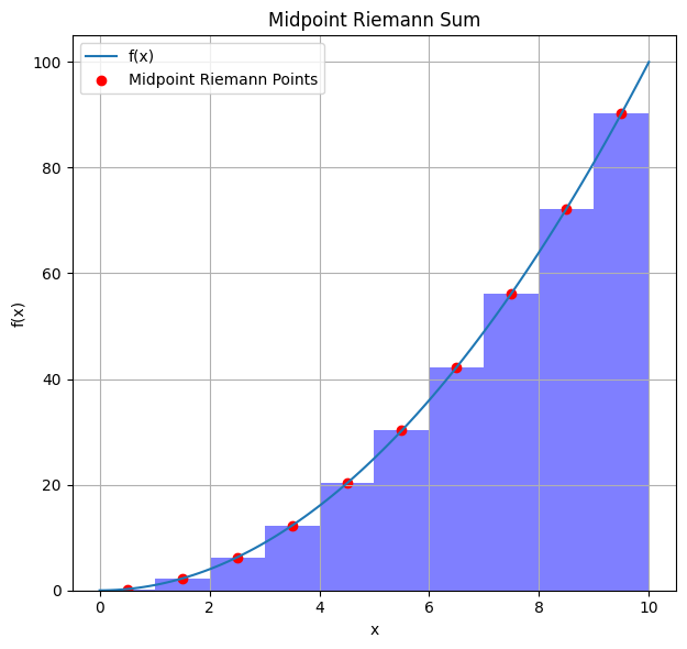
True integral, 1/3 x^3 = 333. Left integral,  285.0 Right integral,  385.0 Midpoint integral,  332.5

Another example, approximate \(\int_0^\pi \sin(x) = 2\)

However, if you have discrete data in the range \([a,b]\) you will not be able to stricly calculate the integral since you would overlap on either side…

Error

The error can be deduced considering the Taylor series of \(f(x)\) around \(y_i\), which as before becomes,

\[\begin{split} \begin{align} f(x) &= f(y_i) + f^{\prime}(y_i)(x - y_i) + \frac{f''(y_i)(x - y_i)^2}{2!} + \cdots \\ \int_{x_i}^{x_{i+1}} f(x) dx &= \int_{x_i}^{x_{i+1}} \left(f(y_i) + f^{\prime}(y_i)(x - y_i) + \frac{f''(y_i)(x - y_i)^2}{2!} + \cdots\right) dx, \\ &= \int_{x_i}^{x_{i+1}} f(y_i)dx + \int_{x_i}^{x_{i+1}} f^{\prime}(y_i)(x - y_i)dx + \int_{x_i}^{x_{i+1}} \frac{f''(y_i)(x - y_i)^2}{2!}dx + \cdots. \end{align} \end{split}\]

but now there is a trick! Since \(x_i\) and \(x_{i+1}\) are symmetric about \(y_i\), all odd derivatives integrate to zero; e.g. \(\int_{x_i}^{x_{i+1}} f^{\prime}(y_i)(x - y_i)dx = 0\)

Therefore the midpoint rule becomes:

\[\int_{x_i}^{x_{i+1}} f(x) dx= hf(y_i) + O(h^3)\]

which has \(O(h^3)\) accuracy for one subinterval or \(O(h^2)\) over the whole interval.