Solvability#
Some systems of equations don’t have a solution, or they do but it’s not unique.
You are organizing a fundraising event and need to buy chairs and tables. Chairs cost $20 each and tables cost $50 each. You have a budget of $700 and need a total of 20 pieces of furniture (chairs and tables combined). How many chairs and tables should you buy?
import sys
sys.path.append('../Tools')
from module import LinearSystemSolverPlotly
---------------------------------------------------------------------------
ImportError                               Traceback (most recent call last)
Cell In[1], line 3
      1 import sys
      2 sys.path.append('../Tools')
----> 3 from module import LinearSystemSolverPlotly

File ~/work/ENGPHYS_3NM4/ENGPHYS_3NM4/Book/Chapters/Linear systems/../Tools/module.py:185
    178         # Final layout
    179         self.fig.update_layout(
    180             title=dict(text=msg, font=dict(color=color)),
    181             xaxis=dict(range=[x_min, x_max]),
    182             yaxis=dict(range=[y_min, y_max])
    183         )
--> 185 LinearSystemSolverPlotly()

File ~/work/ENGPHYS_3NM4/ENGPHYS_3NM4/Book/Chapters/Linear systems/../Tools/module.py:27, in LinearSystemSolverPlotly.__init__(self)
     24 self.toggle_button.observe(self._on_toggle, names='value')
     26 # Plotly figure widget
---> 27 self.fig = go.FigureWidget()
     28 self.fig.update_layout(
     29     width=600, height=600,
     30     margin=dict(l=40, r=40, b=40, t=40),
   (...)     33     showlegend=True
     34 )
     36 # Build 3 equation rows and track the third

File ~/.local/lib/python3.12/site-packages/plotly/missing_anywidget.py:13, in FigureWidget.__init__(self, *args, **kwargs)
     12 def __init__(self, *args, **kwargs):
---> 13     raise ImportError("Please install anywidget to use the FigureWidget class")

ImportError: Please install anywidget to use the FigureWidget class
A system with one solution#
Let \(c\) and \(t\) be the number of chairs and tables respectively. The budget and pieces equations are,
(1) \(20 c + 50 t = 700\)
(2) \( c+t = 20\)
There are a few ways to solve these equations.
Solve graphically#
Since these are lines, let’s plot them!
# prompt: Plot the two lines with a grid

import matplotlib.pyplot as plt
import numpy as np
# Define the x values
x = np.linspace(0, 20, 100)

# Calculate the y values for the first equation (20c + 50t = 700)
y1 = (700 - 20 * x) / 50

# Calculate the y values for the second equation (c + t = 20)
y2 = 20 - x

# Plot the lines
plt.plot(x, y1, label='20c + 50t = 700')
plt.plot(x, y2, label='c + t = 20')

# Add labels and title
plt.xlabel('Number of Chairs (c)')
plt.ylabel('Number of Tables (t)')
plt.title('Fundraising Event')

# Add a grid
plt.grid(True)

# Add a legend
plt.legend()

# Display the plot
plt.show()
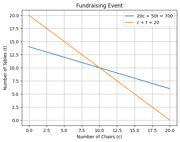
The point where the lines intersect satisfy both equations and is therefore a solution. Since lines only cross once, it is the unique solution.
Solve through elimination#
Multiply the second equation, (2), by \(20\):
(3) \(20c+20t = 400\).
Subtract (3) from (1) and simplify:
\(30t = 300\)
\(t=10\)
Substitute answer into (2):
\(c = 10\)
Matrix formulation and solution#
Writting these as a matrix equation becomes:
\(\begin{pmatrix} 20 & 50 \\ 1 &1 \end{pmatrix} \begin{pmatrix} c \\ t \end{pmatrix} = \begin{pmatrix} 700 \\ 20 \end{pmatrix}\)
or in standard form,
\(A x = b\)
with \(A = \begin{pmatrix} 20 & 50 \\ 1 &1 \end{pmatrix}\)
\(x = \begin{pmatrix} c \\ t \end{pmatrix}\)
\(b = \begin{pmatrix} 700 \\ 20 \end{pmatrix}\)
Let’s find \(A^{-1}\) such that \(x = A^{-1}b\). For a square matrix of dimensions 2x2:
\(\begin{pmatrix} a & b \\ c & d \end{pmatrix}^{-1} = \frac{1}{|A|} \begin{pmatrix} d & -b \\ -c & a \end{pmatrix}\)
where \(|A| = ad-bc\) is the determinant.
The prefactor of \(\frac{1}{|A|}\) is systemic to inversion. In general, \(A^{-1} = \frac{1}{|A|} adj(A)\) for square matricies of any dimension.
For our case,
\(|A| = -30\), and
\(A^{-1} = \frac{1}{-30} \begin{pmatrix} 1 & -50 \\ -1 & 20 \end{pmatrix}\)
thus, \(A^{-1} b\):
\(x = \begin{pmatrix} 10 \\ 10 \end{pmatrix} \)
Infinite solutions#
Lets tweak our problem and see what happens.
There is now a discount on tables down to $20 each. The customer heard about it and cut your budget to $400.
The problem is now:
\(20 c + 20 t = 400\)
\( c+t = 20\)
Graphically#
# prompt: Plot the two lines with a grid making the first line thicker

import matplotlib.pyplot as plt
import numpy as np
# Define the x values
x = np.linspace(0, 20, 100)

# Calculate the y values for the first equation (20c + 20t = 400)
y1 = (400 - 20 * x) / 20

# Calculate the y values for the second equation (c + t = 20)
y2 = 20 - x

# Plot the lines
plt.plot(x, y1, label='20c + 20t = 400', linewidth=3)  # Make the first line thicker
plt.plot(x, y2, label='c + t = 20')

# Add labels and title
plt.xlabel('Number of Chairs (c)')
plt.ylabel('Number of Tables (t)')
plt.title('Fundraising Event (Revised)')

# Add a grid
plt.grid(True)

# Add a legend
plt.legend()

# Display the plot
plt.show()
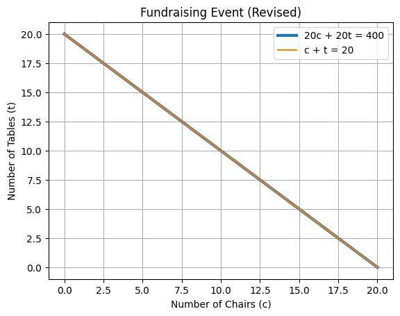
The lines overlap! What does this mean?
Elimination#
Multiple second row by 20:
\(20c+20t = 400\)
subtracting the first we get,
\(0=0\)
:-(
Solve the second equation to find \(c = 20/t\)
and that’s it! For all \(t\) there is a \(c\) that is a solution!
The matrix equation#
\(|A| = ad−bc = 0\)
What does this mean for the inverse \(A^{-1}\)?
No solutions#
WOOPS! The customer meant to say $500; no more, no less!
The problem is now
\(20 c + 20 t = 500\)
\( c+t = 20\)
Graphically#
# prompt: Graph it again please!

import matplotlib.pyplot as plt
import numpy as np
# Define the x values
x = np.linspace(0, 20, 100)

# Calculate the y values for the first equation (20c + 20t = 500)
y1 = (500 - 20 * x) / 20

# Calculate the y values for the second equation (c + t = 20)
y2 = 20 - x

# Plot the lines
plt.plot(x, y1, label='20c + 20t = 500', linewidth=3)  # Make the first line thicker
plt.plot(x, y2, label='c + t = 20')

# Add labels and title
plt.xlabel('Number of Chairs (c)')
plt.ylabel('Number of Tables (t)')
plt.title('Fundraising Event (Revised Again)')

# Add a grid
plt.grid(True)

# Add a legend
plt.legend()

# Display the plot
plt.show()
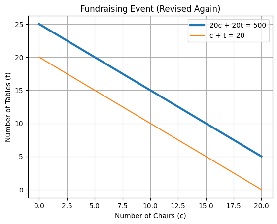
Now they are parralel! What does THIS mean?
Elimination#
The second row multiplied by 20 is still \(20c+20t = 400\) (!!). Now subtracting the first becomes:
\(20c + 20t = 500\)
-\(20c - 20t = -400\)
\(-----------------\)
\(0+0=100\)
… >:-(
And the matrix equation?#
Unchanged since only \(b\) has change!
(What does this tell you?!?)
Putting it together#
Linear equations (in 2 unkowns) are lines in 2D. The solution is the intersection of those lines. 2 Lines can intersect either
in one place (the first example)
everywhere (the second example)
nowhere (the third example)
For 2 and 3, these lines are parallel, i.e. you can slide one to lie ontop of the other.Such lines are called linearly dependent.
Example 1 has linear independent equations which intersect in one place and can be solved.
Scenarios 1 and 2 are called a consistent linear system since an answer can be obtained. Scenario 3 is inconsistent since there is no solution.
The matrix interpretation#
The coefficient matrix \(A\) depends on the nature of the lines, not the constant. When
\(|A| = 0\),
The matrix \(A\) is termed singular. The lines are parallel, which means the equations / rows in \(A\) and linear dependant and you will not be able to solve for a unique \(x\).
This is true regardless of the values of \(b\)!
Approaching singularity#
The matrix interpretation is troubling. The solvability of these systems is related to \(det(A)\) and we have 2 data points:
\(|A| = -30\) and the system is solvable.
\(|A| = 0\) and the system is unsolvable.
What is the significance of \(-30\)? What happens when \(|A| \rightarrow 0\) ?
We saw \(|A| \rightarrow 0\) when we adjusted the price of tables. Let’s play with that! Set the cost of tables to \(20-\epsilon\).
\(20 c + [20+\epsilon] t = 700\)
\( c + t = 20\)
from which we can find,
\(|A| = 20-20+\epsilon = \epsilon\)
which is obviously problematic for small \(\epsilon\)
If we say \(c = 20-t\) and substitute into the first equation:
\( 20 [20 -t] + [20-\epsilon] t = 700\)
\(\epsilon t= 300\)
\( t = 300 / \epsilon\).
Playing with \(\epsilon\) we get,
\(\epsilon\) |
t |
c |
|---|---|---|
-30 |
10 |
10 |
-10 |
30 |
-10 |
-1 |
300 |
-280 |
0.1 |
3000 |
-2980 |
1e-20 |
3e+22 |
-3e+22 |
0 |
\(\infty\) |
\(-\infty\) |
which shows the solution is both increasing but also with an increasing rate!
This should sound alarm bells!
Recall \(\epsilon \sim 10^{-20}\) is well within the range of roundoff error. Here, even just recording the matrix element value can cause astronomical changes in the solution!
These coefficients typically have some uncertainty which compounds the numberical uncertainty.