Linear least squares regression - Pseudoinverse#
Let’s return to linear systems again.
Given a matrix system,
where \(A\) is an \(m\times n\) matrix, \(x\) is \(n\), and \(b\) is \(m\). We cannot solve this for an exact \(x\) with our normal techniques since \(A\) is rectangular, not square.
Recalling the residual is \(\vec{r} = A\vec{x}-\vec{b}\), let’s broaden our concept to a ‘solution’ to say we want to minimize the (norm of the) residual:
This is equivilant to finding the minimum of the surface:
Setting \(\frac{df}{d\vec{x}} = \vec{0}\), we get:
where \(A^†=[A^T A]^{-1} A^T\) is called the (Moore-Penrose) pseudoinverse of \(A\). The pseudoinverse is defined for any rectangular matrix. Note \(A^T A\) is necessarily square, and is generally invertible.
Terminology
A consistent system of equations has a solution that satisfies all the equations.
An inconsistent system has no solution that satisfies all equations simultaneously.
Overdetermined systems have more equations that unknowns which is typical of curve fitting. These systems are inconsistent in that there is no simultaneous solution, but a solution does exists that simultaneously minimizes the error.
Underdetermined systems have fewer equations than unknowns and are also inconsistent but with an infinite number of solutions. E.g.: Parallel lines / 2 equations with 3 variables.
Some properties of the pseudoinverse:
The pseudoinverse is defined for any rectangular matrix
For overconstrained systems using it to solve \(Ax=b\) it results in the best fit (in the least squares sense)
For underconstrained systems it results in a parameterized solution.
The pseudoinverse also covers indefiniate matricies (linearly dependent rows)
Since the ultimate minimum is \(0\), the pseudoinverse is the true inverse for an exactly solvable system.
For these reasons, the pseudoinverse is commonly used to generalize the inverse in analytic derivations (e.g.: to singular matricies), however its application is subtle and the nullspace of the matrix must be considered.
Conditioning of a rectangular matrix#
The pseudoinverse can easily be used to extend the condition number definition to rectangular matricies.
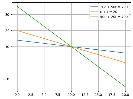
Example: An overdetermined, consistent linear system#
\(20 c + 50 t = 700\)
\( c+t = 20\)
\( 50 c + 20 t = 700\)
which gives the linear system:
#Plot it!

import matplotlib.pyplot as plt
import numpy as np

# Define the x values
x = np.linspace(0, 20, 100)

# Calculate the y values for the first equation (20c + 50t = 700)
y1 = (700 - 20 * x) / 50

# Calculate the y values for the second equation (c + t = 20)
y2 = 20 - x

# Calculate the y values for the third equation (50c + 20t = 700)
y3 = (700 - 50 * x) / 20

# Plot the lines
plt.plot(x, y1, label='20c + 50t = 700')
plt.plot(x, y2, label='c + t = 20')
plt.plot(x, y3, label='50c + 20t = 700')

# Add a grid
plt.grid(True)
plt.legend()
plt.show()
#The arrays are:
# ~~ Question - what is the linear system and how do we solve it?

A = np.array([[20, 50], [1, 1], [50, 20]])
b = np.array([700, 20, 700])

x = np.linalg.solve(A, b)

# Breaks!
---------------------------------------------------------------------------
LinAlgError                               Traceback (most recent call last)
Cell In[2], line 7
      4 A = np.array([[20, 50], [1, 1], [50, 20]])
      5 b = np.array([700, 20, 700])
----> 7 x = np.linalg.solve(A, b)
      9 # Breaks!

File ~/.local/lib/python3.12/site-packages/numpy/linalg/_linalg.py:457, in solve(a, b)
    384 """
    385 Solve a linear matrix equation, or system of linear scalar equations.
    386
   (...)    454
    455 """
    456 a, _ = _makearray(a)
--> 457 _assert_stacked_square(a)
    458 b, wrap = _makearray(b)
    459 t, result_t = _commonType(a, b)

File ~/.local/lib/python3.12/site-packages/numpy/linalg/_linalg.py:264, in _assert_stacked_square(*arrays)
    261     raise LinAlgError('%d-dimensional array given. Array must be '
    262             'at least two-dimensional' % a.ndim)
    263 if m != n:
--> 264     raise LinAlgError('Last 2 dimensions of the array must be square')

LinAlgError: Last 2 dimensions of the array must be square
This doesn’t work since hte matrix is rectangular. But now let’s use the pseudoinverse:
A = np.array([[20, 50], [1, 1], [50, 20]])
b = np.array([700, 20, 700])

M = np.linalg.inv(A.T @ A)@A.T
print('Manual calculation', M, '\n')
print('Package implementation ', np.linalg.pinv(A), '\n')
print('Residual check', M-np.linalg.pinv(A), '\n')
print('Best fit solution', M@b)
Manual calculation [[-0.00952672  0.000204    0.02380661]
 [ 0.02380661  0.000204   -0.00952672]]

Package implementation  [[-0.00952672  0.000204    0.02380661]
 [ 0.02380661  0.000204   -0.00952672]]

Residual check [[-1.73472348e-18  2.71050543e-19  6.93889390e-18]
 [ 1.04083409e-17 -3.25260652e-19 -1.73472348e-18]]

Best fit solution [10. 10.]
Example: An overdetermined, inconsistent linear system#
\(2 c + t = 15\)
\( c + t = 10\)
\( c + 2 t = 14\)
A = np.array([[2, 1], [1, 1], [1, 2]])
b = np.array([15, 10, 14])

x_lsq = np.linalg.pinv(A)@b
print(x_lsq)
x_lsq,_,_,_ = np.linalg.lstsq(A,b)
print(x_lsq)

# Calculate the y values for the first equation (2c + 1t = 15)
y1 = (15 - 2 * x) / 1

# Calculate the y values for the second equation (1c + 1t = 10)
y2 = 10 - x

# Calculate the y values for the third equation (1c + 2t = 14)
y3 = (14 - 1 * x) / 2

# Plot the lines
plt.plot(x, y1, label='2c + 1t = 15')
plt.plot(x, y2, label='1c + 1t = 10')
plt.plot(x, y3, label='1c + 2t = 14')

plt.plot(x_lsq[0], x_lsq[1], 'ro', label='Least Squares Solution')
plt.xlabel('c')
plt.ylabel('t')
plt.title('Least Squares Solution for Inconsistent System')
plt.legend()
plt.grid(True)
plt.xlim(4, 6)
plt.ylim(4, 6)
plt.show()
[5.36363636 4.36363636]
[5.36363636 4.36363636]
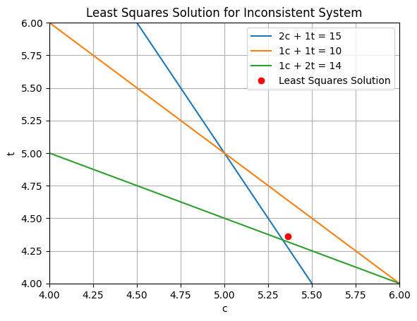
The solution found minimizes the perpendicular distance from each line.
Example: An overdetermined, inconsistent linear system#
\(20 c + 50 t = 700\)
\( c+t = 20\)
\( 60 c + 20 t = 700\)
import matplotlib.pyplot as plt
import numpy as np

# Define the x values
x = np.linspace(7, 10, 100)

# Calculate the y values for the first equation (20c + 50t = 700)
y1 = (700 - 20 * x) / 50

# Calculate the y values for the second equation (c + t = 20)
y2 = 20 - x

# Calculate the y values for the third equation (60c + 20t = 700)
y3 = (700 - 60 * x) / 20

# Plot the lines
plt.plot(x, y1, label='20c + 50t = 700')
plt.plot(x, y2, label='c + t = 20')
plt.plot(x, y3, label='60c + 20t = 700')

plt.xlabel('c')
plt.ylabel('t')
plt.title('Least Squares Solution for Inconsistent System')
plt.legend()
plt.grid(True)
plt.show()

Where do you think he solution is going to be?
A = np.array([[20, 50], [1, 1], [60, 20]])
b = np.array([700, 20, 700])

#np.linalg.(A, b)
x_lsq = np.linalg.pinv(A)@b
print(x_lsq)
x_lsq,_,_,_ = np.linalg.lstsq(A,b)
print(x_lsq)

# Plot the lines
plt.plot(x, y1, label='20c + 50t = 700')
plt.plot(x, y2, label='c + t = 20')
plt.plot(x, y3, label='60c + 20t = 700')


plt.plot(x_lsq[0], x_lsq[1], 'ro', label='Least Squares Solution')
plt.xlabel('c')
plt.ylabel('t')
plt.title('Least Squares Solution for Inconsistent System')
plt.legend()
plt.grid(True)
plt.show()
[ 8.07704251 10.76953789]
[ 8.07704251 10.76953789]
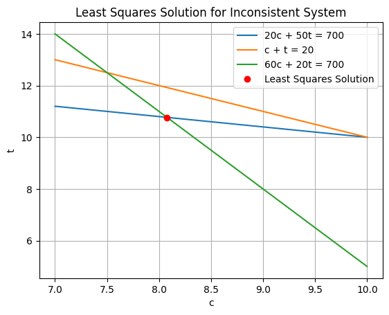
Was this what you were expecting?