Package tools

Scipy implements a number of algorithms for calcualting the eigendecomposition:

\[A = V \Lambda V^{-1}\]

where

• \(V\) is the matrix whose columns are the eigenvectors

• \(\Lambda\) is a diagonal matrix with the eigenvalues on the diagonal

Variants only calculate the eigenvalues (faster) or take advantage of symmetries / sparsity, and numerical stability.

Method	Type	Use Case
eig	Dense (general matrix)	Computes all eigenvalues and eigenvectors of a square matrix.
eigvals	Dense (general matrix)	Computes only eigenvalues of a square matrix (faster than eig).
eigh	Dense (symmetric/Hermitian)	Computes eigenvalues and eigenvectors for symmetric or Hermitian matrices (numerically stable).
eigvalsh	Dense (symmetric/Hermitian)	Computes only eigenvalues of symmetric or Hermitian matrices (faster than eigh).
eigsh	Sparse (symmetric/Hermitian)	Computes a subset of eigenvalues and eigenvectors for sparse symmetric or Hermitian matrices.
eigs	Sparse (general matrix)	Computes a subset of eigenvalues and eigenvectors for sparse general (non-symmetric) matrices.

Eigendecomposition is sometimes called diagonalization.

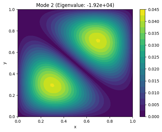
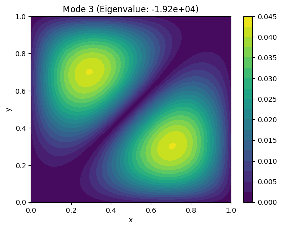
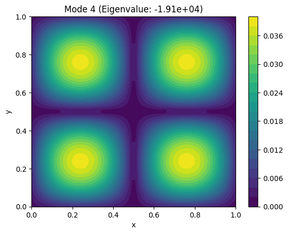
Example: Find the fundamental vibrational modes of a square membrane.

The vibrational modes are solutions to the Laplace equation: $\( \nabla^2 u = 0 \quad u=0 \ on \ boundary\)$

import numpy as np
import matplotlib.pyplot as plt
from scipy.linalg import eigh

# Grid properties
Lx = 1.0  # Length in the x-direction
Ly = 1.0  # Length in the y-direction
Nx = 50   # Number of grid points in the x-direction
Ny = 50   # Number of grid points in the y-direction

dx = Lx / (Nx - 1)  # Grid spacing in the x-direction
dy = Ly / (Ny - 1)  # Grid spacing in the y-direction

# Construct the Laplacian operator for the 2D grid
def construct_laplacian_2d(Nx, Ny, dx, dy):
    N = Nx * Ny
    laplacian = np.zeros((N, N))

    for i in range(N):
        laplacian[i, i] = -2 / dx**2 - 2 / dy**2

        if i % Nx != 0:  # Left neighbor
            laplacian[i, i - 1] = 1 / dx**2
        if (i + 1) % Nx != 0:  # Right neighbor
            laplacian[i, i + 1] = 1 / dx**2
        if i >= Nx:  # Top neighbor
            laplacian[i, i - Nx] = 1 / dy**2
        if i < N - Nx:  # Bottom neighbor
            laplacian[i, i + Nx] = 1 / dy**2

    return laplacian

# Construct the Laplacian matrix
laplacian = construct_laplacian_2d(Nx, Ny, dx, dy)

# Solve the eigenvalue problem
eigenvalues, eigenvectors = eigh(laplacian)

# Extract the first few modes
modes = 4
eigenfunctions = [eigenvectors[:, i].reshape(Nx, Ny) for i in range(modes)]

# Plot the first few eigenfunctions (vibration modes)
for i, eigenfunction in enumerate(eigenfunctions):
    plt.figure()
    plt.contourf(np.linspace(0, Lx, Nx), np.linspace(0, Ly, Ny), abs(eigenfunction), 20, cmap="viridis")
    plt.colorbar()
    plt.title(f"Mode {i+1} (Eigenvalue: {eigenvalues[i]:.2e})")
    plt.xlabel("x")
    plt.ylabel("y")
    plt.show()