Quantifying Error#
import numpy as np
from numpy import cos, sin, abs
import matplotlib.pyplot as plt
True Absolute Error#
The True Absolute Error is the absolute difference between the true value and an approximation.
\(E_t = |\text{True} - \text{Approximate}|\)
This metric is only useful when the true value is known.
Example: What is the derivative of \(\sin(x)\) at \(x=0\)?#
Recall the definition of a derivative:
\(\frac{d}{dx} \sin(x) = \lim_{\Delta x \to 0} \frac{\sin(x+\Delta x) - \sin(x)}{\Delta x}\)
The true value of the derivative of \(\sin(x)\) is \(\cos(x)\).
value_true = cos(0)
print(f"The true value is: {value_true}")
The true value is: 1.0
We can define a function to approximate the derivative using a finite \(\Delta x\):
def approx_derivative(delta_x):
    """Approximates the derivative of sin(x) at x=0."""
    return (sin(0 + delta_x) - sin(0)) / delta_x
For \(\Delta x = 0.1\), the approximate value is:
value_approx = approx_derivative(delta_x=0.1)
print(f"The approximate value is: {value_approx}")
The approximate value is: 0.9983341664682815
The true absolute error is therefore:
E_t = abs(value_true - value_approx)
print(f"The true absolute error is: {E_t}")
The true absolute error is: 0.0016658335317184525
True Relative Error#
Often, the absolute error is not as useful as the True Relative Error, because it does not account for the magnitude of the value. For example, a 1-meter error in GPS is insignificant for a long road trip but critical for a self-driving car.
The true relative error is defined as:
\(\epsilon_t = \frac{E_t}{\text{True}}\)
or as a percentage:
\(\epsilon_t (\%) = \frac{E_t}{\text{True}} \times 100\%\)
Example: What is the relative error from the previous calculation?#
eps_t = E_t / value_true
print(f"The true relative error is: {eps_t}")
The true relative error is: 0.0016658335317184525
Approximate Absolute and Relative Error#
What if we don’t know the true value? Numerical methods often have a tunable parameter that controls accuracy (like \(\Delta x\) above). We can estimate the error by comparing sequential approximations, using the better approximation in place of the true value.
\(E_a = |\text{Better approximation} - \text{Approximation}|\)
\(\epsilon_a = \frac{E_a}{\text{Better approximation}}\)
Example: Use a smaller step size to find the approximate error.#
approx_1 = approx_derivative(0.1)
approx_2 = approx_derivative(0.01)

E_a = abs(approx_2 - approx_1)
epsilon_a = E_a / approx_2

print(f"The approximate absolute error is: {E_a}")
print(f"The approximate relative error is: {epsilon_a}")
The approximate absolute error is: 0.0016491669483849059
The approximate relative error is: 0.001649194434821387
Note the two appear similar because the true value is 1. In general these may be orders of magnitude different.
Tolerance#
Since we often don’t know the true answer, we can never be certain that we have reached it. Instead, we can determine when the answer is no longer improving significantly.
In programming, we define a tolerance to determine when the error is small enough.
Absolute Tolerance (\(Tol_a\)): The threshold below which the absolute error is considered acceptable.
Relative Tolerance (\(Tol_r\)): The threshold below which the relative error is considered acceptable.
Pseudocode Concept#
parameter = initial_value
while True:
    result = run_algorithm(parameter)
    error = calculate_error(result, previous_result)
    if error < tolerance:
        break
    parameter = reduce_parameter(parameter)
Example: Exploring \(E_a\) and \(\epsilon_a\) as a function of \(\Delta x\)#
delta_x = np.logspace(0, -10, 11)
E_a = np.zeros(delta_x.size)
epsilon_a = np.zeros(delta_x.size)

for i, dx in enumerate(delta_x):
    # Note: We are comparing the approximation at dx with the one at dx/10
    E_a[i] = abs(approx_derivative(dx/10) - approx_derivative(dx))
    epsilon_a[i] = E_a[i] / approx_derivative(dx/10)

plt.loglog(delta_x, abs(E_a), marker='o', label='$E_a$')
plt.loglog(delta_x, abs(epsilon_a), marker='s', label='$\epsilon_a$')
plt.xlabel('$\Delta x$')
plt.ylabel('Error')
plt.legend()
plt.grid(True)
plt.show()
<>:11: SyntaxWarning: invalid escape sequence '\e'
<>:12: SyntaxWarning: invalid escape sequence '\D'
<>:11: SyntaxWarning: invalid escape sequence '\e'
<>:12: SyntaxWarning: invalid escape sequence '\D'
/tmp/ipykernel_3752/2221679652.py:11: SyntaxWarning: invalid escape sequence '\e'
  plt.loglog(delta_x, abs(epsilon_a), marker='s', label='$\epsilon_a$')
/tmp/ipykernel_3752/2221679652.py:12: SyntaxWarning: invalid escape sequence '\D'
  plt.xlabel('$\Delta x$')
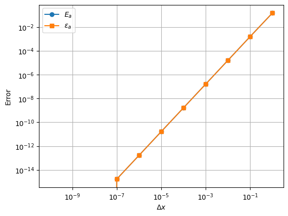
Observations:
The two error curves overlap. Why?
The plot is a straight line on a log-log scale. What does this imply?
There is a sharp drop-off in the error around \(10^{-8}\). What could be causing this?