Polynomial interpolation

Polynomial interpolation#

Polynomial interpolation is a straightforward approach to interpolation.

Three methods to obtain polynomials are established here. For a given set of data, they all must result in the same polynomial. The difference is the means by which they are achieved, which translates to the ways that they are used.

Lagrange Polynomial Interpolation#

Legendre polynomial interpolation constructs the Legendre polynomial as,

\[ y(x) = \sum_{i = 1}^n y_i P_i(x) \]

which is a weighted sum of the Lagrange basis polynomials, $P_i(x)$,

\[ P_i(x) = \prod_{j = 1, j\ne i}^n\frac{x - x_j}{x_i - x_j}. \]

N.B.: $\prod$ means the product of, like $\sum$ means the sum of.

Lagrange basis polynomials#

By construction,

$P_i(x_j) = 1$ when $i = j$
$P_i(x_j) = 0$ when $i \ne j$.

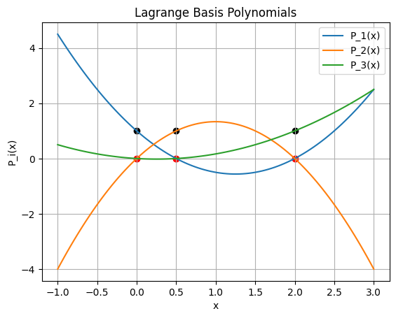
Example: Find and plot the Lagrange basis polynomials#

Use the data: x = [0, .5, 2] y = [1, 3, 2]

(9)#\[\begin{eqnarray} P_1(x) &=& \frac{(x - x_2)(x - x_3)}{(x_1-x_2)(x_1-x_3)} = \frac{(x - 1)(x - 2)}{(0-1)(0-2)} = \frac{1}{2}(x^2 - 3x + 2),\\ P_2(x) &=& \frac{(x - x_1)(x - x_3)}{(x_2-x_1)(x_2-x_3)} = \frac{(x - 0)(x - 2)}{(1-0)(1-2)} = -x^2 + 2x,\\ P_3(x) &=& \frac{(x - x_1)(x - x_2)}{(x_3-x_1)(x_3-x_2)} = \frac{(x - 0)(x - 1)}{(2-0)(2-1)} = \frac{1}{2}(x^2 - x). \end{eqnarray}\]

Plot each polynomial and verify the property that $P_i(x_j) = 1$ when $i = j$ and $P_i(x_j) = 0$ when $i \ne j$.

import numpy as np
import matplotlib.pyplot as plt
from numpy.polynomial import legendre

# Data points
x = [0, .5, 2]
y = [1, 3, 2]

# Calculate the Lagrange basis polynomials
n = len(x)
P = []
for i in range(n):
  numerator = 1
  denominator = 1
  for j in range(n):
    if i != j:
      numerator = np.polymul(numerator, np.poly1d([1, -x[j]]))
      denominator = denominator * (x[i] - x[j])
  P.append(np.poly1d(np.polydiv(numerator, denominator)[0]))


# Plot the Lagrange basis polynomials
x_plot = np.linspace(-1, 3, 100)

for i in range(n):
    y_plot = P[i](x_plot)
    plt.plot(x_plot, y_plot, label=f'P_{i+1}(x)')

plt.scatter(x, [1] * len(x), color='black')
plt.scatter(x, [0] * len(x), color='red')
plt.scatter(x, [0] * len(x), color='red')

plt.xlabel('x')
plt.ylabel('P_i(x)')
plt.title('Lagrange Basis Polynomials')
plt.legend()
plt.grid(True)
plt.show()

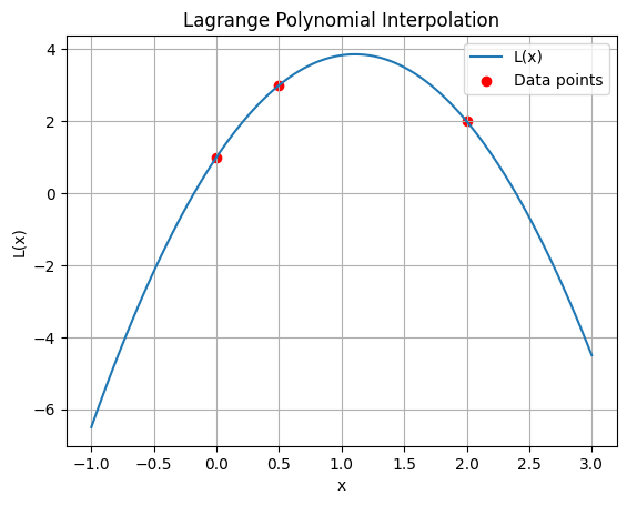
../../../_images/9d720e8bf8eedeb1efcee32ba8479af075187f7f0406bedabfa7c686a21aed28.png

Assembling the polynomial#

Since $P_{i\ne j}=0$, and $P_{i = j}=1$, it is trivial to see that for $ y(x) = \sum_{i = 1}^n \omega_i P_i(x) $, the coefficients are simply:

\[ y(x) = \sum_{i = 1}^n y_i P_i(x) \]

import matplotlib.pyplot as plt
import numpy as np
# Construct the Lagrange polynomial
L = np.poly1d(0)
for i in range(n):
  L = L + y[i] * P[i]

# Plot the Lagrange polynomial
y_plot = L(x_plot)
plt.plot(x_plot, y_plot, label='L(x)')
plt.scatter(x, y, color='red', label='Data points')
plt.xlabel('x')
plt.ylabel('L(x)')
plt.title('Lagrange Polynomial Interpolation')
plt.legend()
plt.grid(True)
plt.show()

../../../_images/61912b1e454de0613e59fafaf0b60bc3457cae640a3a6bebd7b2804844684ed7.png

Analysis#

We can observe some notes:

For $n$ data points we necessarily produce a unique polynominal that crosses each one.
If we have two measurements at the same input, $x_i = x_j$, $P_i =\sim \frac{1}{0}$ which is undefined unless $x_i=x_j$ and $y_i=y_j$ in which case the data pair is redundant and can be removed.
Each evalulation of $P(x)$ involves $n-1$ products, and $L(x)$ is the sum of $n$ bases, therefore evaluation is $O(n^2)$
Adding new data means restarting the compuation.

import sympy as sp

x = [0, 1, 2, 3, 4]
y = [1, 3, 2, 5, 7]

n = len(x)
x_sym = sp.Symbol('x')

L = 0
for i in range(n):
    term = y[i]
    for j in range(n):
        if i != j:
            term *= (x_sym - x[j]) / (x[i] - x[j])
    L += term


print(L)

print('which is an ugly way of writing out:')
print(L.simplify())

3*x*(4/3 - x/3)*(3/2 - x/2)*(2 - x) + x*(2 - x/2)*(3 - x)*(x - 1) + 5*x*(4 - x)*(x/2 - 1/2)*(x - 2)/3 + 7*x*(x/3 - 1/3)*(x/2 - 1)*(x - 3)/4 + (1 - x)*(1 - x/2)*(1 - x/3)*(1 - x/4)
which is an ugly way of writing out:
-x**4/2 + 25*x**3/6 - 21*x**2/2 + 53*x/6 + 1

Error#

It can be shown that the error in the interpolation is,

\[ y^{true}(x)-y(x) = \frac{[x-x_1][x-x_2][x-x_3]...[x-x_n]}{(n+1)!} f^{(n+1)}(\xi) \]

where $\xi$ is in the interval $(x_0, x_n)$.

Since for $n$ datapoints there is a unique polynomial of degree $n-1$, which can be expressed as a Lagrange polynomial, this analysis is universal to all polynomial interpolations!. The main takeaway is that:

The further a data point is from $x$, the more it contributes to the error.

Barycentric Lagrange Interpolation#

Let’s try to improve the performance of Lagrange Interpolation. Let:

\[ \Omega(x) = \prod_{j = 1}^n [x - x_j] \]

and the barycentric weights, $w_i$:

\[ w_i = \prod_{j = 1, j\ne i}^n\frac{1}{x_i - x_j}. \]

and write:

\[ P_i(x) = \Omega(x) \frac{w_i}{x - x_j}. \]

and factor the $\Omega$ out of the sum:

\[ y(x) = \Omega(x) \sum_{j = 1}^n \frac{w_i}{x - x_j} y_i. \]

which is $O(n)$ for evaluation. Calculation of $w_i$ can be formulated recursively, such that each $w_i$ takes $O(n)$ and the full takes $O(n^2)$ with updates n.

NB: The weights depend only on $x_i$, not $y_i$ - this means if we are measuring multiple functions on the same spacing, we can reuse the weights, leading to substantial computaitonal savings. The benefit being that the calucation of the $\omega_i$, $O(n^2)$ is precomputed.

Barycentric formula#

We can write one more form which is commonly implemented. Let’s add one more piece of data:

\[ 1 = \sum_{j=0}^n P_j = \Omega(x) \sum_{j=0}^n \frac{w_j}{x-x_j}\]

then we divide the previous function and write:

\[ y(x) = \frac{\sum_{j = 0}^n \frac{w_i}{x - x_j} y_i}{\sum_{j = 0}^n \frac{w_i}{x - x_j}} \]

where we have cancelled $\Omega$! Besides elegance, his avoids an issue when evaluating $x\rightarrow x_i$ where roundoff can cause subtractive cancellation. Since the term appears in the numerator and denominator this cancels out!

Newton’s divided difference method#

Newton’s polynomial interpolation has the form:

\[ y(x) = a_0 + a_1[x-x_0] + a_2 [x-x_0][x-x_1] + \dots + a_n[x-x_0][x-x_1]\dots[x-x_n]\]

which has the advantage of $O(n)$ evaluations due to recursion and nested multiplication. E.g. for 4 terms,

\[ y(x) = a_0 + [x-x_0] \bigg[a_1 + [x-x_1] \big[a_2 + [x-x_2] a_3 \big] \bigg] \]

Newton’s method is also known as the divided differences

This was the algorithm was used to calculate function tables like logarithms and trignometry functions. It was then the basis for the difference engine, an early mechanical calculator.

Let’s pick a data point to start at. Say $y(x_0) = a_0 = y_0$, $$a_0 = y_0$$

Add the next data point: $y(x_1) = a_0 + a_1(x_1-x_0) = y_1$, or:

\[a_1 = \frac{y_1 - y_0}{x_1 - x_0}\]

Now, insert data point $(x_2, y_2)$,

\[a_2 = \frac{\frac{y_2 - y_1}{x_2 - x_1} - \frac{y_1 - y_0}{x_1 - x_0}}{x_2 - x_0}\]

and similarly,

\[a_3 = \frac{\frac{\frac{y_3-y_2}{x_3-x_2} - \frac{y_2 - y_1}{x_2-x_1}}{x_3 - x_1} - \frac{\frac{y_2-y_1}{x_2-x_1}-\frac{y_1 - y_0}{x_1 - x_0}}{x_2-x_0}}{x_3 - x_0}\]

Notice the recurrsion and the division of the differences.

Let’s generalize this. Define the two-argument function:

\[ y[x_1, x_0] = \frac{y_1 - y_0}{x_1 - x_0}\]

and the ternary recursively:

\[ y[x_2, x_1, x_0] = \frac{\frac{y_2 - y_1}{x_2 - x_1} - \frac{y_1 - y_0}{x_1 - x_0}}{x_2 - x_0} = \frac{y[x_2,x_1] - y[x_1,x_0]}{x_2-x_1}\]

The $n-nary$ function is:

\[ y[x_k, x_{k-1}, \dots, x_{1}, x_0] = \frac{y[x_k, x_{k-1}, \dots, x_{2}, x_2] - y[x_{k-1}, x_{k-2}, \dots, x_{1}, x_0]}{x_k-x_0}\]

We can visualize this is in a tableau: $$ \begin{array}{cccccc} x_0 & y_0 \\ & & y[x_1,x_0] \\ x_1 & y_1 & & y[x_2, x_1,x_0]\\ & & y[x_2,x_1] & & y[x_3, x_2, x_1,x_0]\\ x_2 & y_2 & & y[x_3, x_2,x_1] & & y[x_4, x_3, x_2, x_1,x_0]\\ & & y[x_3,x_2] & & y[x_4, x_3, x_2, x_1]\\ x_3 & y_3 & & y[x_4, x_3,x_2]\\ & & y[x_4,x_3] \\ x_4 & y_4 \end{array} $$

where element is the difference of the two to the left. Alternately, it is sometimes written in the form,

\[\begin{split} \begin{array}{c||cccccc} x_0 & y_0 & 0 & 0 & 0 & 0\\ x_1 & y_1 & y[x_1,x_0] & 0 & 0 & 0\\ x_2 & y_2 & y[x_2,x_1] & y[x_2, x_1,x_0] & 0 & 0 \\ x_3 & y_3 & y[x_3,x_2] & y[x_3, x_2,x_1] & y[x_3, x_2, x_1,x_0] & 0 \\ x_4 & y_4 & y[x_4,x_3] & y[x_4, x_3,x_2] & y[x_4, x_3, x_2, x_1] & y[x_4, x_3, x_2, x_1,x_0] \end{array} \end{split}\]

Note that the diagonal is the coefficients that we need, i.e. $a_0, a_1, a_2, a_3, a_4$ for the polynomial.

Notes:

The order that the datapoints are added is arbitrary but will result in a different tableau (with the same diagonal).
We can build this matrix / tableau diagonal-by-diagonal which means adding new data points doesn’t require recalculation of the others.
Each new diagonal (datapoint) takes $O(n)$ so assembly of the tableau takes $~O(n^2)$.
Evaluation of f(x) takes $O(n)$
These coefficients are independant of $x$

Direct solution#

Lastly, there is a direct solution method that only became really practical with the advent of modern computing since it focusses on linear systems:

Consider a general, $n$ th order polynomial,

\[ y(x) = a_n x^n + a_{n-1} x^{n-1} \dots a_2 x^2 + a_1 x +a_0\]

since

\[y(x_i) = a_n x_i^n + a_{n-1} x_i^{n-1} \dots a_2 x_i^2 + a_1 x_i +a_0 = y_i\]

we can write out in matrix form,

\[\begin{split} \begin{bmatrix} 1 & x_1 & x_1^2 & \cdots & x_1^m \\ 1 & x_2 & x_2^2 & \cdots & x_2^m \\ \vdots & \vdots & \vdots & \ddots & \vdots \\ 1 & x_n & x_n^2 & \cdots & x_n^m \end{bmatrix} \begin{bmatrix} a_0 \\ a_1 \\ a_2 \\ \vdots \\ a_m \end{bmatrix} = \begin{bmatrix} y_1 \\ y_2 \\ y_3 \\ \vdots \\ y_n \end{bmatrix} \end{split}\]

where the matrix of coefficients is called a Vandermonde matrix. This system can be solved for $a_i$ with a dense linear solver. The issue with this method is that the system is notoriously ill-conditioned and roundoff error accumulates rapidly for large $n$.

Example: Interpolate our toy problem#

Let us know examine our toy problem. Since all the polynomial interpolation functions generate the same unique polynomial, any will suffice:

import matplotlib.pyplot as plt
import numpy as np

# Define the function
def f(x):
  return np.exp(-(x/2)**2)

# Create x values for plotting
x_toy = np.linspace(-6, 6, 100)
y_toy = f(x_toy)

# Sample 11 random points in the range -5 to 6
x_d = np.arange(-5, 6, 1)
y_d = f(x_d)

# Interpolate using numpy Legendre
from numpy.polynomial import legendre
coefficients = legendre.legfit(x_d, y_d, len(x_d) - 1)
legendre_polynomial = legendre.Legendre(coefficients)

# Create x values for plotting the interpolated polynomial
x_interp = np.linspace(-5.5, 5.5, 200)
y_interp = legendre_polynomial(x_interp)

# Plot the original curve, sampled points, and interpolated polynomial
plt.plot(x_toy, y_toy, label='exp(-(x/2)^2)')
plt.scatter(x_d, y_d, color='red', label='Sampled points')
plt.plot(x_interp, y_interp, label='Legendre Interpolation')
plt.xlabel('x')
plt.ylabel('y')
plt.legend()
plt.title('Function, Sampled Points, and Legendre Interpolation')
plt.grid(True)
plt.show()

../../../_images/9ca8d4783ed713630b58c6b75a6c3be97c7e0688e5c715207136caade97892c0.png

YIKES!

This is an example of Runge’s phenomenon: That even for a seeminlgly ideal case of equally spaced samples, higher order polynomials can show huge oscillations between samples!