Root finding

The roots (aka zeros) of a function are values of function arguments forwhich the function is zero:

Find \(x\) such that:

\[ f(x) = 0 \]

It can become complicated when we consider vector \(\vec{x}\) and even \(\vec{f}\), but consider a special case of finding the roots of \(\vec{f}(\vec{x})\) is our familiar linear system, \(A \vec{x} -\vec{b} = \vec{0}\). Solving linear systems is a special case of root finding, which is generalized to nonlinear functions.

Roots of some nonlinear functions

Let’s build some intuition by exploring some type of roots in 1D functions using the graphical method: Plot the function and examine where it crosses the x-axis.

NB: Note the structure of the code below - Since we don’t know a priori where the roots will be, we have to take a series of initial guesses and cross our finger…. and even then we may fail to find them all!

import numpy as np
import matplotlib.pyplot as plt
from scipy.optimize import root

def plot_and_find_roots(func):
    x = np.linspace(-10, 10, 400)
    y = func(x)

    # Find roots
    x0s = np.arange(-10, 10, 1)
    roots = []
    for x0 in x0s:
        r = root(func, x0=x0)
        if r.success:
            roots.append((r.x[0], r.fun[0]))

    # Remove duplicate roots (within tolerance)
    unique_roots = []
    tol = 1e-6
    for rx, ry in roots:
        if not any(abs(rx - ux) < tol for ux, _ in unique_roots):
            unique_roots.append((rx, ry))

    # Plot with Matplotlib
    plt.figure(figsize=(8, 5))
    plt.plot(x, y, label='f(x)')
    plt.axhline(0, color='black', linestyle='--', label='x-axis')
    if unique_roots:
        plt.scatter([rx for rx, _ in unique_roots], [0]*len(unique_roots), color='red', s=60, label='Roots')
    plt.title('Plot of f(x) and its Roots')
    plt.xlabel('x')
    plt.ylabel('f(x)')
    plt.xlim(-10, 10)
    plt.ylim(-10, 10)
    plt.legend()
    plt.grid(True)
    plt.show()

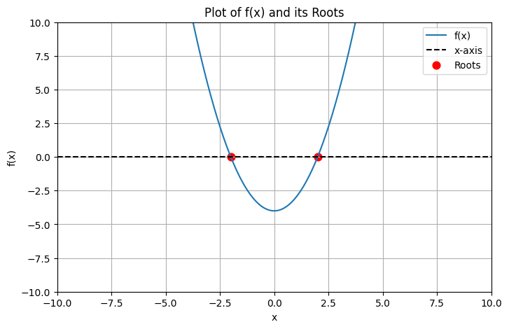
Example 1: Real roots - \(x^2-4\)

plot_and_find_roots(lambda x: x**2-4)

Example 2: No roots - \(1/x\)

plot_and_find_roots(lambda x: 1/x)

/tmp/ipykernel_3536/3010058334.py:1: RuntimeWarning: divide by zero encountered in divide
  plot_and_find_roots(lambda x: 1/x)

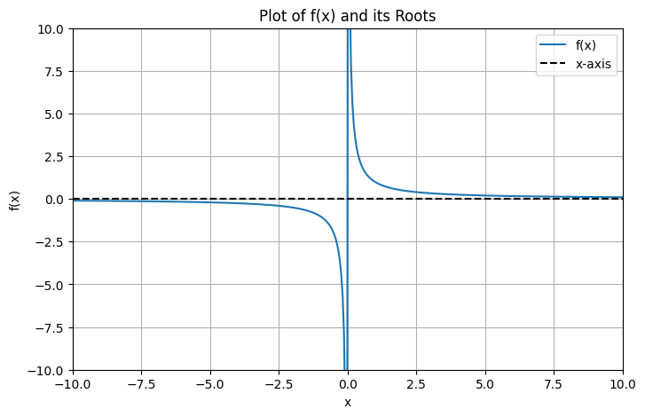
(Noting that the vertical line is a plotting artifact).

Example 3: Infinite roots \(sin(x^2)\)

plot_and_find_roots(lambda x: np.sin(x**2))

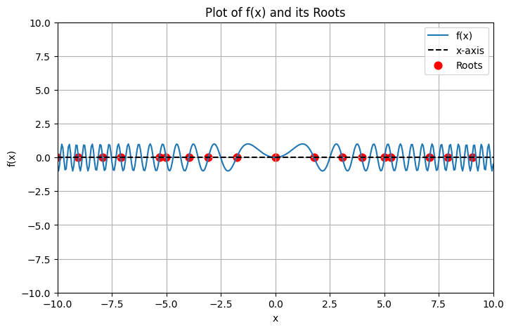
Only the roots closest to the initial guesses are found!

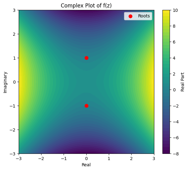
Complex roots - \(x^2+1\)

Even the graphical method is not completely reliable due to the existence of complex roots

def fun(x):
    return x**2 + 1

# Wrong!
plot_and_find_roots(fun)

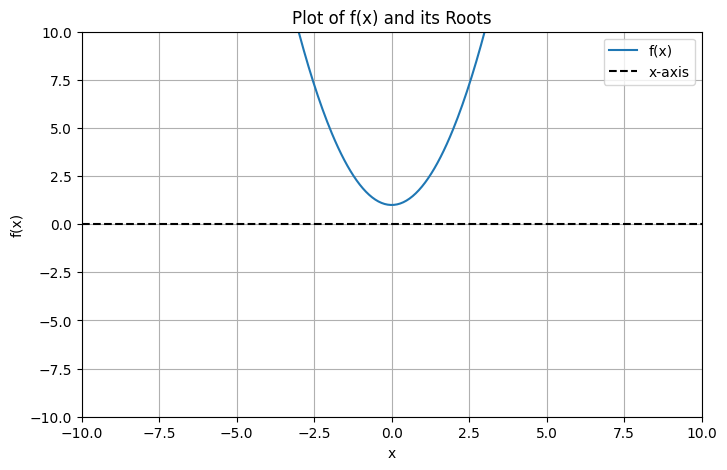
But this is wrong! The quadratic has 2 roots but we need to use a different method:

root(lambda x: x**2+1, x0 = [1+1j, 1-1j], method = "krylov")

 message: A solution was found at the specified tolerance.
 success: True
  status: 1
     fun: [1.6870727e-11-2.00208702e-11j 1.6870727e-11+2.00208702e-11j]
       x: [-1.00104351e-11+1.j -1.00104351e-11-1.j]
     nit: 6
  method: krylov
    nfev: 16

import numpy as np
import matplotlib.pyplot as plt
from scipy.optimize import root

def complex_plot(func):
    real_range = np.linspace(-3, 3, 100)
    imag_range = np.linspace(-3, 3, 100)
    real_part = np.empty((len(real_range), len(imag_range)))

    for i, real in enumerate(real_range):
        for j, imag in enumerate(imag_range):
            z = complex(real, imag)
            result = func(z)
            real_part[i, j] = result.real

    # Find roots
    r = root(lambda x: x**2 + 1, x0=[1 + 1j, 1 - 1j], method="krylov")
    root_x = [root_val.real for root_val in r.x] if r.success else []
    root_y = [root_val.imag for root_val in r.x] if r.success else []

    # Plot with Matplotlib
    plt.figure(figsize=(7, 6))
    X, Y = np.meshgrid(real_range, imag_range, indexing='ij')
    cp = plt.contourf(X, Y, real_part, levels=50, cmap='viridis')
    plt.colorbar(cp, label='Real Part')
    if root_x:
        plt.scatter(root_x, root_y, color='red', s=60, label='Roots')
    plt.title('Complex Plot of f(z)')
    plt.xlabel('Real')
    plt.ylabel('Imaginary')
    plt.legend()
    plt.show()

# Use the function to plot x**2 + 1
complex_plot(lambda z: z**2 + 1)

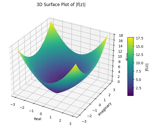
# 3D surface plot of the absolute value of f(z) over the complex plane
import matplotlib.pyplot as plt
from mpl_toolkits.mplot3d import Axes3D
import numpy as np

def complex_surface_plot(func):
    real_range = np.linspace(-3, 3, 100)
    imag_range = np.linspace(-3, 3, 100)
    abs_val = np.empty((len(real_range), len(imag_range)))

    for i, real in enumerate(real_range):
        for j, imag in enumerate(imag_range):
            z = complex(real, imag)
            result = func(z)
            abs_val[i, j] = abs(result)

    X, Y = np.meshgrid(real_range, imag_range, indexing='ij')

    fig = plt.figure(figsize=(8, 6))
    ax = fig.add_subplot(111, projection='3d')
    surf = ax.plot_surface(X, Y, abs_val, cmap='viridis')
    fig.colorbar(surf, ax=ax, shrink=0.5, aspect=10, label='|f(z)|')
    ax.set_title('3D Surface Plot of |f(z)|')
    ax.set_xlabel('Real')
    ax.set_ylabel('Imaginary')
    ax.set_zlabel('|f(z)|')
    plt.show()

# Example: 3D surface plot for x**2 + 1
complex_surface_plot(lambda z: z**2 + 1)

DON’T WORRY - We won’t be dealing with complex numbers in general in this course :-)

Pathalogical / well-behaved functions

Some functions can be very tricky indeed, such as the Weierstrass Function,

\[\begin{split} \sum_{n=0}^\infty a^n cos (b^n \pi x) \\ 0<a<1 \\ a b > 1+\frac{3 \pi}{2} \end{split}\]

which looks like:

This is a classic example of a continuous but nowhere differentiable function! It is a fractal, and yet roots do exist and may be on interest. It is a classic example of a pathalogical function.

Different appliations will have different criteria for pathalogical vs well behaved functions, and no general definition exists although there is seldom dissagreement amoung non-mathematicians about which is which.

Generally, well behaved functions don’t have sharp corners, singularities, discontinuities, etc.